[Classic Paper Review] Optimal Impulsive Collision Avoidance in Low Earth Orbit
2026-06-23
Optimal Impulsive Collision Avoidance in Low Earth Orbit
Paper: Claudio Bombardelli and Javier Hernando-Ayuso, "Optimal Impulsive Collision Avoidance in Low Earth Orbit", Journal of Guidance, Control, and Dynamics, Vol. 38, No. 2, 2015. DOI: 10.2514/1.G000742
Affiliation: Universidad Politécnica de Madrid
1. Introduction
As the population of space objects in Earth orbit continues to grow, Collision Avoidance Maneuvers (CAM) have become an indispensable part of satellite operations. By 2025, over 40,000 cataloged debris objects larger than 10 cm populate Earth orbit, and the number of conjunction alerts issued annually is measured in tens of thousands. Each predicted close approach may require a spacecraft to perform an orbital maneuver to reduce collision risk.
The core problem of collision avoidance can be stated as: Given a fixed velocity impulse budget ($\Delta v$), in which direction should the maneuver be applied to maximize the avoidance effect? The difficulty lies in:
- Highly nonlinear orbital dynamics
- A continuous 3D space of possible maneuver directions
- High-dimensional integrals for collision probability computation
- Varying orbital parameters across different conjunction scenarios
Traditional methods rely on numerical propagation and parameter scanning, requiring minutes to hours of computation — far too slow for rapid decision-making. Bombardelli and Hernando-Ayuso's 2015 paper reduces the optimal CAM problem to closed-form analytical solutions with sub-millisecond computation time, marking a paradigm shift in the field of space debris collision avoidance.
2. Theoretical Foundation: The b-Plane and Collision Probability
2.1 The b-Plane Coordinate System
To describe the close approach of two space objects, the paper employs the b-plane coordinate system $\langle \xi, \eta, \zeta \rangle$, centered on the target spacecraft S2:
$$ \mathbf{u}_\xi = \frac{\mathbf{v}_2 \times \mathbf{v}_1}{\| \mathbf{v}_2 \times \mathbf{v}_1 \|} $$
$$ \mathbf{u}_\eta = \frac{\mathbf{v}_1 - \mathbf{v}_2}{\| \mathbf{v}_1 - \mathbf{v}_2 \|} $$
$$ \mathbf{u}_\zeta = \mathbf{u}_\xi \times \mathbf{u}_\eta $$
where $\mathbf{v}_1$ and $\mathbf{v}_2$ are the velocity vectors of the maneuverable spacecraft S1 and the target S2, respectively. $\mathbf{u}_\eta$ points along the relative velocity direction, and the b-plane (the $\xi$-$\zeta$ plane) is perpendicular to the relative velocity. The closest approach point projects to position $(\xi_e, 0, \zeta_e)$ on the b-plane.
2.2 Analytical Collision Probability
Under the short-term encounter hypothesis, the relative motion can be approximated as uniform rectilinear. The collision probability reduces to a 2D integral on the b-plane:
$$ P = \iint_A \frac{1}{2\pi\sigma_\xi\sigma_\zeta\sqrt{1-\rho_{\xi\zeta}^2}} \exp\left[-\frac{1}{2(1-\rho_{\xi\zeta}^2)}\left(\frac{\xi-\xi_e}{\sigma_\xi}\right)^2 + \left(\frac{\zeta-\zeta_e}{\sigma_\zeta}\right)^2 - 2\rho_{\xi\zeta}\frac{(\zeta-\zeta_e)(\xi-\xi_e)}{\sigma_\zeta\sigma_\xi}\right] d\xi d\zeta $$
where $A$ is the circular region of radius $s_A$ (the combined cross-sectional radius of both objects), and $\sigma_\xi, \sigma_\zeta, \rho_{\xi\zeta}$ are extracted from the relative position covariance matrix $C_{\xi\zeta}$ in b-plane axes.
Using Chan's method [Chan, 2008], this integral reduces to a Rician integral:
$$ P(u, v) = e^{-v/2} \sum_{m=0}^{\infty} \frac{v^m}{2^m m!} \left[1 - e^{-u/2} \sum_{k=0}^{m} \frac{u^k}{2^k k!}\right] $$
where:
$$ u = \frac{s_A^2}{\sigma_\xi\sigma_\zeta \sqrt{1-\rho_{\xi\zeta}^2}} $$
$$ v = \frac{\left(\frac{\xi_e}{\sigma_\xi}\right)^2 + \left(\frac{\zeta_e}{\sigma_\zeta}\right)^2 - 2\rho_{\xi\zeta}\frac{\xi_e}{\sigma_\xi}\frac{\zeta_e}{\sigma_\zeta}}{1-\rho_{\xi\zeta}^2} $$
Here $u$ is the ratio of the impact cross-sectional area to the area of the 1-$\sigma$ covariance ellipse, and $v$ is the square of the "depth of intrusion" [Lázaro & Righetti, 2012].
3. Key Breakthrough: The Linear Model
3.1 Linear Relation Between b-Plane Displacement and Impulse
One of the paper's core innovations is a linearized model building on Bombardelli's earlier work [2013]. After applying an impulse $\Delta v = (\Delta v_r, \Delta v_\theta, \Delta v_h)^T$ (radial, transversal, out-of-plane components) at the maneuver point, the relative position change on the b-plane is:
$$ \mathbf{r} = \mathbf{R} \mathbf{K} \mathbf{D} \Delta v \equiv \mathbf{M} \Delta v $$
where the three matrices describe the geometric transformation, orbital kinematics transformation, and maneuver position transformation, respectively.
3.2 Physical Meaning of the Matrices
Matrix $\mathbf{R}$ (geometric rotation) transforms the impulse from S1's orbital frame to the b-plane:
$$ \mathbf{R} = \begin{bmatrix} 0 & 0 & -1 \\ \cos\beta & -\sin\beta & 0 \\ -\sin\beta & -\cos\beta & 0 \end{bmatrix} $$
where $\beta$ is the angle between $\mathbf{v}_1$ and $\mathbf{v}_1 - \mathbf{v}_2$.
Matrix $\mathbf{K}$ encodes the orbital parameters (semi-major axis $a_0$, eccentricity $e_0$, true anomaly at conjunction $\theta_c$, etc.) and the encounter geometry (orbital plane difference $\phi$, relative velocity orientation $\psi$). It is the key link between impulse direction and b-plane displacement.
Matrix $\mathbf{D}$ contains the orbital propagation from the maneuver time $\theta_m$ to the conjunction time $\theta_c$. Its elements — $d_{tr}, d_{t\theta}, d_{rr}, d_{r\theta}, d_{wh}$ — are nonlinear functions of $e_0, \theta_c$, and $\theta_m$ (see Appendix A of the paper).
4. Maximum Miss Distance Maneuver
4.1 Problem Formulation
For the direct impact case ($r_e = 0$), the maximum miss distance optimization problem is:
$$ \begin{aligned} \text{maximize} \quad & J_r(\Delta v) = \xi^2 + \zeta^2 \\ \text{subject to} \quad & f(\Delta v) = \Delta v^T \Delta v - \Delta v_0^2 \leq 0 \end{aligned} $$
Rewriting in matrix form:
$$ J_r = \mathbf{r}^T \mathbf{Q} \mathbf{r} = \Delta v^T \mathbf{A} \Delta v $$
where $\mathbf{Q} = \text{diag}(1, 0, 1)$ selects only the $\xi$ and $\zeta$ components (the b-plane), and $\mathbf{A} = \mathbf{M}^T \mathbf{Q} \mathbf{M}$.
4.2 Reduction to an Eigenvalue Problem
Using the method of Lagrange multipliers:
$$ \mathcal{L}(\Delta v, \lambda) = J_r - \lambda f $$
Setting $\partial\mathcal{L}/\partial\Delta v = 0$ yields:
$$ \mathbf{A} \Delta v = \lambda \Delta v $$
This is a standard eigenvalue problem. The optimal maneuver direction is the eigenvector $\mathbf{s}_1$ corresponding to the largest eigenvalue $\lambda_1$ of matrix $\mathbf{A}$.
The optimal impulse is:
$$ \Delta v_{\text{opt}} = \Delta v_0 \mathbf{s}_1 $$
And the corresponding maximum miss distance:
$$ \Delta r_{\max} = \sqrt{\lambda_1} \Delta v_0 $$
A critical finding: $\text{rank}(\mathbf{A})$ is either 1 (when $\theta_c - \theta_m = 2\pi n$) or 2 (in general). This means there is always at least one impulse direction that leaves the miss distance unchanged (corresponding to the zero eigenvalue).
5. Minimum Collision Probability Maneuver
For minimizing collision probability, the objective becomes:
$$ \tilde{J}_P = v = \frac{\xi^2}{\sigma_\xi^2} + \frac{\zeta^2}{\sigma_\zeta^2} - 2\rho_{\xi\zeta} \frac{\xi\zeta}{\sigma_\xi\sigma_\zeta} \bigg/ (1-\rho_{\xi\zeta}^2) $$
Writing this as a quadratic form:
$$ \tilde{J}_P = \mathbf{r}^T \mathbf{Q}' \mathbf{r} $$
where:
$$ \mathbf{Q}' = \frac{1}{1-\rho_{\xi\zeta}^2} \begin{bmatrix} 1/\sigma_\xi^2 & 0 & -\rho_{\xi\zeta}/\sigma_\xi\sigma_\zeta \\ 0 & 0 & 0 \\ -\rho_{\xi\zeta}/\sigma_\xi\sigma_\zeta & 0 & 1/\sigma_\zeta^2 \end{bmatrix} $$
Substituting $\mathbf{r} = \mathbf{M}\Delta v$:
$$ \tilde{J}_P = \Delta v^T \mathbf{A}' \Delta v $$
This again reduces to the eigenvalue problem $\mathbf{A}'\Delta v = \lambda \Delta v$, with the optimal solution corresponding to the eigenvector of the maximum eigenvalue.
The maximum miss distance and minimum collision probability criteria are formally equivalent — they differ only in the quadratic form matrix.
6. General Case: Non-Direct Impact
6.1 Generalized Problem
When the expected miss distance is non-zero ($r_e \neq 0$), the b-plane relative position after maneuver becomes:
$$ \mathbf{r} = \mathbf{r}_e + \mathbf{M} \Delta v $$
The squared miss distance becomes:
$$ J_r = J_{r0} + \Delta v^T \mathbf{A} \Delta v + 2 \mathbf{r}_e^T \mathbf{Q} \mathbf{M} \Delta v $$
This is a non-convex quadratic optimization problem. The paper ingeniously transforms it into a convex one.
6.2 Convexification
Let $\mathbf{u} = \Delta v / \Delta v_0$, $\mathbf{b}^T = \mathbf{r}_e^T \mathbf{Q} \mathbf{M} / \Delta v_0$. The problem becomes:
$$ \begin{aligned} \text{maximize} \quad & \tilde{J}_r(\mathbf{u}) = \mathbf{u}^T \mathbf{A} \mathbf{u} + 2\mathbf{b}^T \mathbf{u} \\ \text{subject to} \quad & \mathbf{u}^T \mathbf{u} - 1 \leq 0 \end{aligned} $$
Following Boyd [2004]'s convex optimization theory, this reduces to:
$$ \text{minimize} \quad \frac{(\mathbf{s}_1^T \mathbf{b})^2}{\lambda - \lambda_1} + \frac{(\mathbf{s}_2^T \mathbf{b})^2}{\lambda - \lambda_2} + \lambda \quad \text{s.t. } \lambda \geq \lambda_1 $$
where $\lambda_1 \geq \lambda_2$ are the two non-zero eigenvalues of $\mathbf{A}$, and $\mathbf{s}_1, \mathbf{s}_2$ are the corresponding eigenvectors.
6.3 Solution Procedure
Step 1: Solve the nonlinear equation (via Newton's method):
$$ \left(\frac{\mathbf{s}_1^T \mathbf{b}}{\lambda - \lambda_1}\right)^2 + \left(\frac{\mathbf{s}_2^T \mathbf{b}}{\lambda - \lambda_2}\right)^2 - 1 = 0, \quad \lambda \geq \lambda_1 $$
Step 2: Compute the optimal impulse:
$$ \Delta v_{\text{opt}} = -\Delta v_0 (\mathbf{A} - \lambda_{\text{opt}} \mathbf{I})^\dagger \mathbf{b} $$
where $\dagger$ denotes the pseudoinverse.
Step 3: Substitute into Eq. (22) to obtain the maximum miss distance.
6.4 Geometric Properties of the Optimal Solution
The paper proves that the optimal solution must satisfy:
$$ \mathbf{r}_e^T \mathbf{Q} (\mathbf{r}_{\text{opt}} - \mathbf{r}_e) \geq 0 $$
This constrains feasible solutions to the half-space bounded by the line perpendicular to the initial b-plane relative position $\mathbf{r}_e$. As the maneuver angular distance $\Delta\theta$ varies, the optimal solution can exhibit discontinuities, which occur when the reachable domain ellipse becomes tangent to the constraint boundary.
7. Case Study I: The 2009 Iridium–Cosmos Collision
7.1 Encounter Geometry
On February 10, 2009, the operational Iridium 33 spacecraft and the defunct Cosmos 2251 satellite collided at approximately 788.6 km altitude over Siberia, generating over 2,000 trackable debris fragments — the first accidental hypervelocity collision between two intact satellites in history.
The paper treats Iridium as the maneuverable spacecraft S1, with the key parameters:
| Parameter | Value | Description |
|---|---|---|
| $a_0$ | 7155.8 km | Semi-major axis |
| $e_0$ | $2 \times 10^{-4}$ | Eccentricity |
| $\phi$ | 180.0° | Orbital plane angle |
| $\psi$ | 77.5° | Relative velocity orientation |
| $\theta_c$ | -16.85° | True anomaly at conjunction |
| $\chi$ | 1.0 | Velocity ratio |
| $s_A$ | 7 m | Combined cross-sectional radius |
Covariance matrix (b-plane):
$$ C_{\xi\zeta} = \begin{bmatrix} 0.02 & 0 \\ 0 & 0.80 \end{bmatrix} \text{km}^2 $$
Non-direct impact assumed: $\xi_e = -70$ m, $\zeta_e = -70$ m.
7.2 Optimal Maneuver Direction
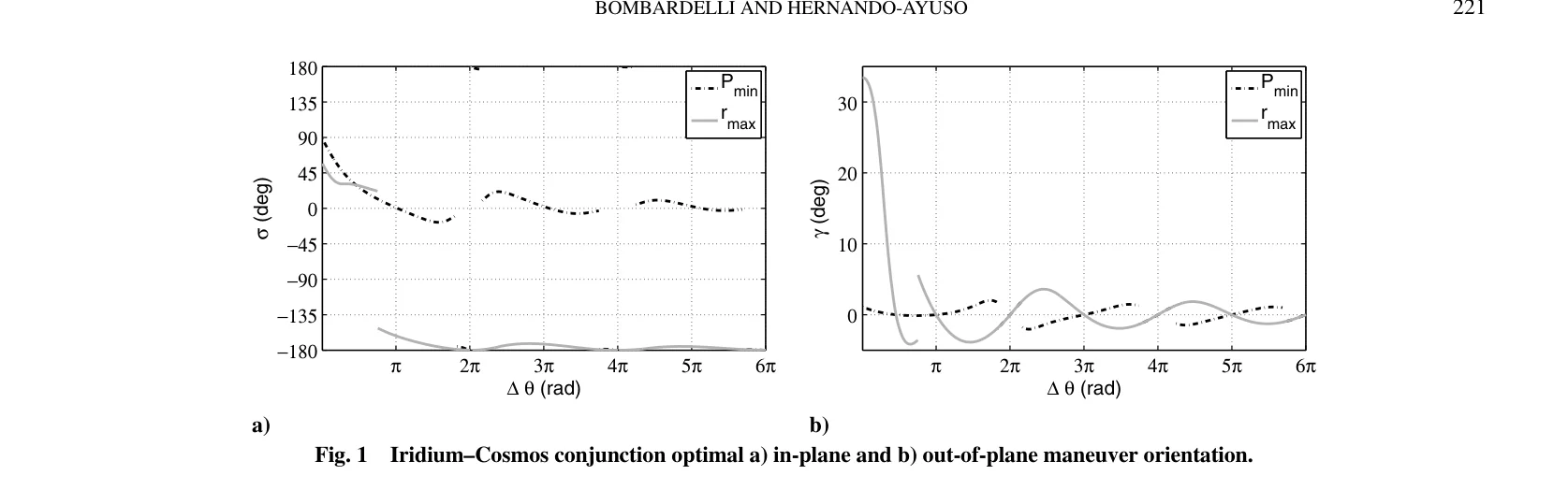
Figure 1 shows the optimal maneuver orientation for the Iridium–Cosmos conjunction. Fig 1(a) shows the in-plane rotation angle $\sigma$, and Fig 1(b) shows the out-of-plane rotation angle $\gamma$. Two curves compare the minimum collision probability ($P_{\min}$, dashed) and maximum miss distance ($r_{\max}$, solid) criteria.
Key findings:
- For small $\Delta\theta$ (maneuvering close to conjunction), both $\sigma$ and $\gamma$ deviate significantly from zero — the optimal impulse is neither purely tangential nor purely normal
- The two criteria differ substantially for small $\Delta\theta$ — they should not be used interchangeably
- As $\Delta\theta \to \infty$ (maneuvering many orbits in advance), the two criteria converge
7.3 Miss Distance and Probability Comparison
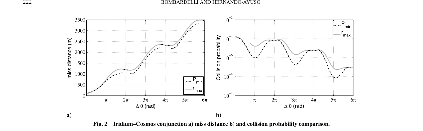
Figure 2 compares the effectiveness under both criteria. Fig 2(a) shows that the $r_{\max}$ criterion achieves miss distances above 3000 m for $\Delta\theta > 2\pi$, while the $P_{\min}$ criterion yields slightly lower values. Fig 2(b) shows the collision probability decreasing with periodic oscillations as $\Delta\theta$ increases.
7.4 b-Plane Reachable Domain
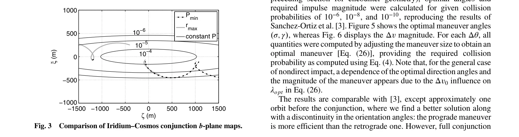
Figure 3 shows the b-plane map comparing the optimal solutions. Constant-probability contours form ellipses, and the two criteria follow different paths in the $\xi$-$\zeta$ plane.
Most importantly, Figure 4 reveals the discontinuity of the optimal solution:
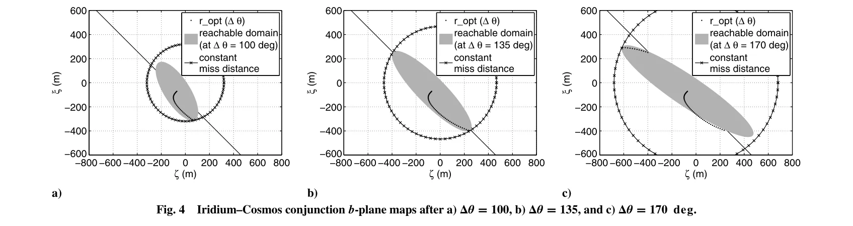
Figure 4 shows the evolution of the reachable domain (gray elliptical region) as $\Delta\theta$ increases from $100^\circ$ to $170^\circ$. When $\Delta\theta \approx 136^\circ$, the major axis of the reachable domain ellipse becomes tangent to the constraint boundary, and the optimal solution undergoes a discontinuous jump. This is not a numerical artifact — it is an intrinsic geometric property of the problem.
8. Case Study II: The RapidEye4–UoSat2 Conjunction
8.1 Encounter Geometry
In May 2013, the RapidEye4 satellite performed an actual collision avoidance maneuver following a predicted conjunction with the non-operational UoSat2 satellite. Key parameters:
| Parameter | Value |
|---|---|
| $a_0$ | 7004.7 km |
| $e_0$ | $1.37 \times 10^{-3}$ |
| $\phi$ | 0° |
| $\psi$ | -26.49° |
| $\theta_c$ | 15.5° |
| $s_A$ | 1.58 m |
8.2 Optimal Maneuver for Given Collision Probability
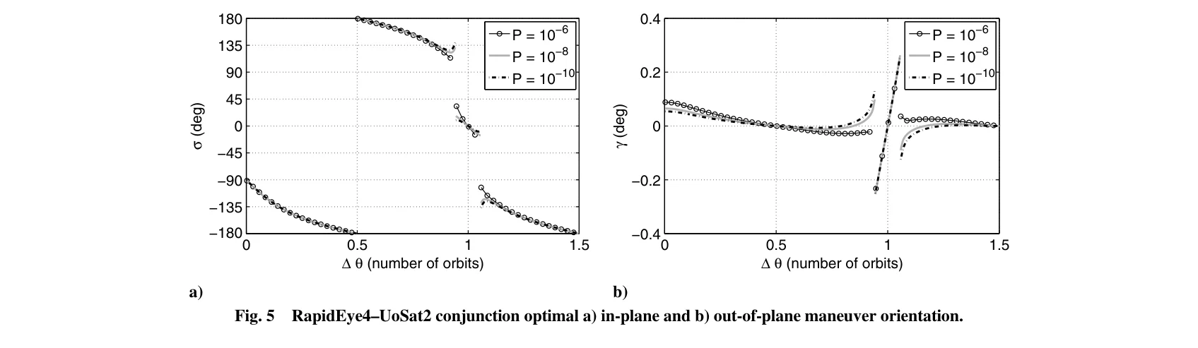
Figure 5 shows the optimal maneuver angles required to achieve specified collision probabilities ($10^{-6}, 10^{-8}, 10^{-10}$). The in-plane angle $\sigma$ (Fig 5a) shows a discontinuous jump near $\Delta\theta = 1$ orbit (from approximately $-90^\circ$ to $180^\circ$), corresponding to the switch from prograde to retrograde maneuvering. The out-of-plane angle $\gamma$ (Fig 5b) exhibits a characteristic spike at the same location.
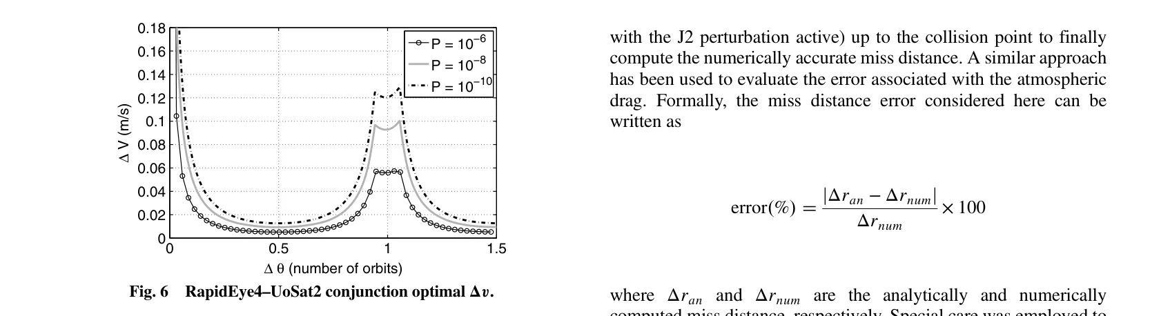
Figure 6 shows the $\Delta v$ magnitude required to achieve each specified collision probability. Key results:
- More stringent requirements (smaller $P$) demand larger $\Delta v$
- As maneuver time approaches conjunction ($\Delta\theta \to 0$), required $\Delta v$ increases dramatically
- For $P = 10^{-6}$, the optimal maneuver requires less than $0.02$ m/s — remarkably efficient
9. Accuracy Assessment
9.1 J2 Perturbation Effects
The paper uses a Keplerian orbit model but evaluates the impact of the dominant J2 Earth gravitational harmonic.
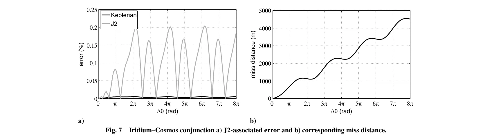
Figure 7(a) shows that for the actual Iridium-Cosmos scenario, the J2-induced miss distance error does not exceed 0.25% — negligible for engineering purposes. Fig 7(b) shows the corresponding miss distance curve.
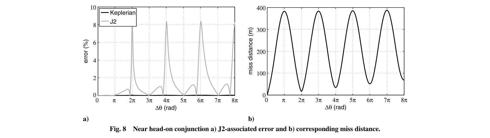
Figure 8 examines a more extreme near head-on collision scenario ($\psi = 1^\circ$, inclination $45^\circ$ to maximize J2 effects). Fig 8(a) shows error peaks reaching 9%, but these peaks coincide with poorly planned maneuvers (regions where Fig 8b shows very low achievable miss distance). In practice, operators would not choose these inefficient maneuvers, so J2 errors are negligible for operational purposes.
The paper further evaluates atmospheric drag effects. Even in extreme cases (350 km altitude, near head-on), the drag-induced error remains small as long as the number of lead orbits is modest.
9.2 Comparison with Other Methods
| Feature | Traditional Numerical | This Analytical Method |
|---|---|---|
| Computation time | Minutes to hours | Sub-millisecond |
| Parameter scanning | Requires 3D grid | Direct optimal solution |
| Accuracy | Numerical integration step-dependent | Same as eigenvalue solver precision |
| Applicability | General | Keplerian + small perturbation corrections |
| Physical insight | Black box | Clear geometric/physical interpretation |
10. Conclusions and Implications
Bombardelli & Hernando-Ayuso (2015) masterfully reduce the complex CAM optimization problem to:
- An eigenvalue problem — computing eigenvalues and eigenvectors of a $3\times 3$ matrix
- A single-variable nonlinear equation — easily solved with Newton's method
This reduction brings the computation time for optimal CAM from minutes down to sub-milliseconds, making it easy to embed in real-time collision avoidance decision systems.
Key takeaways for engineering practice:
-
Near-conjunction maneuver directions are non-intuitive — the optimal impulse is not simply "accelerate along velocity direction" but a combination including out-of-plane components that must be precisely determined via eigenvalue analysis
-
Minimum collision probability ≠ maximum miss distance — the two criteria differ significantly for small $\Delta\theta$; mission risk preferences should guide the choice of optimization objective
-
Analytical model accuracy is sufficient for engineering use — errors from J2 and drag perturbations remain under 1% for well-planned maneuvers, making the analytical approach a viable replacement for costly numerical optimization
-
Open-source tool available — the authors' OCCAM (Optimal Computation of Collision Avoidance Maneuver) tool provides an online demonstration for practical operations and education
This paper represents a paradigm shift from "numerical trial-and-error" to "analytical solution" for space debris collision avoidance. It is essential reading for every researcher and engineer working in space debris, orbital mechanics, and spacecraft operations.
References
-
Bombardelli, C., and Hernando-Ayuso, J., "Optimal Impulsive Collision Avoidance in Low Earth Orbit", J. Guidance, Control, and Dynamics, Vol. 38, No. 2, 2015, pp. 217-225. DOI: 10.2514/1.G000742
-
Bombardelli, C., "Analytical Formulation of Impulsive Collision Avoidance Dynamics", Celestial Mechanics and Dynamical Astronomy, Vol. 118, No. 2, 2013, pp. 99-114.
-
Chan, F. K., Spacecraft Collision Probability, Aerospace Press, El Segundo, CA, 2008.
-
Klinkrad, H., Space Debris: Models and Risk Analysis, Springer–Verlag, New York, 2006.
-
Sanchez-Ortiz, N., et al., "Collision Risk Assessment and Avoidance Manoeuvres — The New CORAM Tool for ESA", 64th IAC, 2013.
-
Boyd, S. P., and Vandenberghe, L., Convex Optimization, Cambridge Univ. Press, 2004.
-
Lázaro, D., and Righetti, P., "Evolution of EUMETSAT LEO Conjunctions Events Handling Operations", 12th SpaceOps, 2012.
-
Valsecchi, G., et al., "Resonant Returns to Close Approaches: Analytical Theory", Astronomy and Astrophysics, Vol. 408, No. 3, 2003, pp. 1179-1196.