[Classic Paper Review] Low-Thrust Collision Avoidance in Circular Orbits
2026-06-24
Low-Thrust Collision Avoidance in Circular Orbits
Paper: Javier Hernando-Ayuso and Claudio Bombardelli, "Low-Thrust Collision Avoidance in Circular Orbits", Journal of Guidance, Control, and Dynamics, Vol. 44, No. 5, 2021, pp. 984–995. DOI: 10.2514/1.G005547
Affiliation: ispace-inc (Tokyo) / Universidad Politécnica de Madrid
1. Introduction
The first post in this series reviewed the landmark work by Bombardelli & Hernando-Ayuso (2015) on impulsive optimal collision avoidance: assuming the spacecraft applies an instantaneous $\Delta v$, the optimization problem is elegantly reduced to an eigenvalue problem of a $3\times3$ matrix. In reality, however, an increasing number of spacecraft are adopting electric propulsion systems — particularly the upcoming large LEO constellations (Starlink, OneWeb, etc.) — which produce continuous, low-thrust rather than instantaneous impulses.
Key differences between impulsive and low-thrust maneuvers:
| Property | Impulsive Maneuver | Low-Thrust Maneuver |
|---|---|---|
| Thrust application | Instantaneous $\Delta v$ | Continuous thrust arc $a_0$ |
| Mathematical problem | Eigenvalue problem + single nonlinear equation | Optimal control → Two-Point Boundary Value Problem (TPBVP) |
| Control variable | Thrust direction (3D vector) | Time-varying thrust direction (function) |
| Solution method | Closed-form analytical | Indirect method + Pontryagin's maximum principle |
| Computational complexity | Sub-millisecond | Requires numerical TPBVP solver |
| Typical propulsion | Chemical | Electric (Hall/Ion thrusters) |
This article reviews the 2021 JGCD paper by Hernando-Ayuso & Bombardelli, which systematically solves the low-thrust collision avoidance optimal control problem in circular orbits for the first time, extending the impulsive framework of their 2015 work into the continuous-thrust domain.
2. Theoretical Foundation: The b-Plane and Collision Probability
2.1 The b-Plane Coordinate System
Consistent with the previous paper, this work employs the b-plane coordinate system $\langle \xi, \eta, \zeta \rangle$ to describe close encounters. Here $\mathbf{u}_\eta$ points along the relative velocity direction, the b-plane ($\xi$-$\zeta$ plane) is perpendicular to the relative velocity, and the $\xi$ axis aligns with the Minimum Orbit Intersection Distance (MOID).
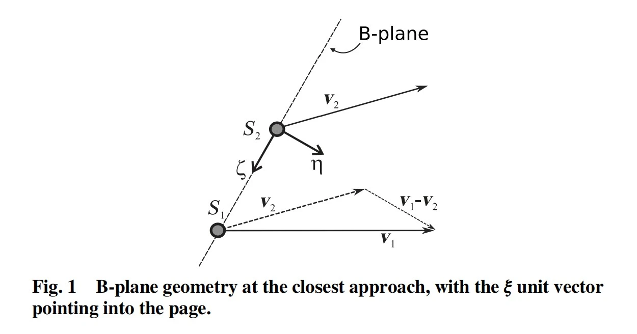
Figure 1 shows the b-plane geometry at closest approach. The $\xi$ unit vector points into the page, and $\zeta$ together with $\eta$ form a right-handed coordinate system. The b-plane position vector of the maneuverable spacecraft S1 relative to the target S2 is $\mathbf{b} = (\xi, \zeta)^T$. The diagram also labels the velocity vectors $\mathbf{v}_1$, $\mathbf{v}_2$ and their relative velocity $\mathbf{v}_1 - \mathbf{v}_2$ — the fundamental geometric framework underlying the entire collision avoidance theory.
2.2 Surrogate Objective for Collision Probability
Under the short-term encounter hypothesis, the paper employs Chan's method (Rician integral) for collision probability computation. A key insight is that collision probability $P$ is a monotonically decreasing function of $v$:
$$v = \frac{\left(\frac{\xi}{\sigma_\xi}\right)^2 + \left(\frac{\zeta}{\sigma_\zeta}\right)^2 - 2\rho_{\xi\zeta}\frac{\xi}{\sigma_\xi}\frac{\zeta}{\sigma_\zeta}}{1-\rho_{\xi\zeta}^2}$$
Therefore, minimizing collision probability is equivalent to maximizing the following surrogate objective:
$$J_P = \left(\frac{\xi}{\sigma_\xi}\right)^2 + \left(\frac{\zeta}{\sigma_\zeta}\right)^2 - 2\rho_{\xi\zeta}\frac{\xi\zeta}{\sigma_\xi\sigma_\zeta}$$
An alternative objective is maximizing the miss distance:
$$J_d = \xi^2 + \zeta^2$$
Both objectives can be expressed as quadratic forms of the b-plane coordinates $J = \frac{1}{2}\mathbf{b}^T \mathbf{Q} \mathbf{b}$, differing only in the structure of the $\mathbf{Q}$ matrix.
3. b-Plane Kinematics for Circular Orbits
3.1 Simplifications from the General Case
In the impulsive model of Bombardelli & Hernando-Ayuso (2015), the maneuverable spacecraft S1 can be on an elliptical orbit of arbitrary eccentricity, requiring the full $\mathbf{R}, \mathbf{K}, \mathbf{D}$ transformation matrices. In this paper, the authors focus on the case where both objects are in circular orbits — a highly relevant scenario for large LEO constellations — greatly simplifying the encounter geometry.
For circular orbits, the velocity magnitudes of the two objects are approximately equal ($\chi \simeq 1$), and the encounter geometry reduces to a single parameter: the mutual orbital plane inclination $\kappa$:
- When $0 < \kappa < \pi/2$: $\phi = 0, \psi = \mp\kappa$
- When $\pi/2 < \kappa < \pi$: $\phi = \pi, \psi = \pi \pm \kappa$
where $\phi$ is the in-plane rotation angle and $\psi$ is the out-of-plane rotation angle.
3.2 Simplified Transformation Matrix
The relationship between b-plane displacement and thrust reduces to a compact $2\times3$ matrix $\mathbf{R}_0$:
$$\mathbf{R}_0 = \begin{bmatrix} 0 & 0 & -1 \\ -\cos\frac{\kappa}{2} & -\sin\frac{\kappa}{2} & 0 \end{bmatrix}$$
This is substantially simpler than the full $3\times3$ matrix $\mathbf{RKD}$ of the impulsive case, laying the groundwork for the low-thrust optimization that follows.
4. Low-Thrust Collision Avoidance Dynamics
4.1 Equations of Motion
Let $\mathbf{u} = (u_r, u_\theta, u_h)^T$ be the thrust acceleration vector (radial, transversal, and out-of-plane components in the orbital frame), with constant magnitude far smaller than the local gravitational acceleration:
$$\sqrt{u_r^2 + u_\theta^2 + u_h^2} = a_0 \ll \frac{\mu}{r_1^2}$$
During the thrust arc, consider an infinitesimal time interval $\delta t$. The velocity variation produced by the thrust, $\delta\mathbf{v} = \mathbf{u}\delta t$, induces a b-plane displacement $\delta\mathbf{b} = (\delta\xi, \delta\zeta)^T$. Using the linear relationship [Bombardelli & Hernando-Ayuso, 2015]:
$$\frac{d\mathbf{b}}{dt} = \mathbf{M}_0(t) \mathbf{u}$$
where $\mathbf{M}_0(t) = \mathbf{R}_0(t) \mathbf{K}(t) \mathbf{D}(t)$ is a $2\times3$ time-varying matrix mapping the thrust direction to b-plane motion.
This is the critical generalization from impulsive to low-thrust: in the impulsive case, $\Delta\mathbf{b} = \mathbf{M}\Delta\mathbf{v}$ is a one-shot algebraic relation; under low thrust, it becomes a differential equation — the control variable $\mathbf{u}(t)$ is a function of time, elevating the optimization complexity from finite to infinite dimensions.
4.2 Maneuver Scheme
The CAM scheme considered in this paper consists of: a continuous thrust arc $\Delta\theta_t > 0$ (constant magnitude), followed by a coast arc $\Delta\theta_c \geq 0$. The thrust arc length is typically constrained by the power availability of electric propulsion systems (often limited to the sunlit fraction of the orbit). Multi-arc maneuvers are not addressed here but could be built via linear superposition of single-arc solutions in future work.
5. Analytical Solution for Tangential Thrust
5.1 Pure Tangential Maneuver
Before diving into optimal control, the authors present an engineer-friendly simplified solution: the thrust direction is held strictly tangential (along or against the velocity direction). Building on the prior work by Bombardelli et al. [2011] on the two-body problem with constant tangential thrust, they derive closed-form expressions for the b-plane coordinates after the thrust arc:
$$\xi \simeq \xi_0 + 2a_0\frac{r_1^3}{\mu}\left[\Delta\theta_t + \sin(\Delta\theta_c) - \sin(\Delta\theta_t + \Delta\theta_c)\right]$$
$$\zeta \simeq \zeta_0 + a_0\frac{r_1^3}{\mu}\cos\frac{\kappa}{2}\left[3\Delta\theta_t + \Delta\theta_t\left(2 + \frac{\Delta\theta_c}{\Delta\theta_t}\right) - 8\sin\frac{\Delta\theta_t}{2}\sin\left(\frac{\Delta\theta_t}{2} + \Delta\theta_c\right)\right]$$
The elegance of these two analytical formulas lies in the fact that no differential equations or optimization routines need to be solved — given the thrust arc length $\Delta\theta_t$ and coast arc length $\Delta\theta_c$, the collision probability can be directly computed. This provides an extremely fast assessment tool for preliminary mission design.
5.2 Characteristics of the Tangential Solution
Note that the $\xi$ coordinate contains a secular term $2a_0(r_1^3/\mu)\Delta\theta_t$, meaning the displacement along $\xi$ (the MOID direction) grows linearly with the thrust arc length — this is the most efficient way to increase miss distance. The $\zeta$ coordinate contains both secular and oscillatory components.
6. Optimal Control Formulation
6.1 Application of Pontryagin's Maximum Principle
The collision avoidance problem is formulated as a Bolza-type optimal control problem. The objective and dynamics are:
$$J = \frac{1}{2}\mathbf{b}^T\mathbf{Q}\mathbf{b}\bigg|_{t=t_f} + \int_{t_0}^{t_f} \boldsymbol{\lambda}^T(t)\mathbf{M}_0(t)\mathbf{u}\,dt$$
The Hamiltonian is constructed as $H(\mathbf{u}, \boldsymbol{\lambda}, t) = \boldsymbol{\lambda}^T\mathbf{M}_0\mathbf{u}$, where $\boldsymbol{\lambda} = (\lambda_\xi, \lambda_\zeta)^T$ is the costate vector.
Applying Pontryagin's maximum principle yields three key results:
- Thrust magnitude must take its maximum value $a_0$ (the continuous-thrust equivalent of bang-bang control)
- The optimal thrust direction is:
$$\mathbf{u} = a_0\frac{\mathbf{M}_0^T\boldsymbol{\lambda}}{\|\mathbf{M}_0^T\boldsymbol{\lambda}\|}$$
- Costate dynamics (since the Hamiltonian does not explicitly depend on $\mathbf{b}$):
$$\frac{d\boldsymbol{\lambda}}{dt} = -\frac{\partial H}{\partial \mathbf{b}} = 0 \quad\Rightarrow\quad \boldsymbol{\lambda}(t) = \text{constant}$$
- Transversality condition: $\boldsymbol{\lambda}(t_f) = \mathbf{Q}\mathbf{b}(t_f)$
6.2 Reduction to a 2D TPBVP
This is the crown jewel of the optimal control derivation. Because the costate vector is constant and linearly related to the terminal b-vector through the $\mathbf{Q}$ matrix, the entire optimization problem reduces to a two-dimensional Two-Point Boundary Value Problem (TPBVP):
$$\frac{d\mathbf{b}}{dt} = a_0\frac{\mathbf{M}_0\mathbf{M}_0^T\mathbf{Q}\mathbf{b}(t_f)}{\|\mathbf{M}_0^T\mathbf{Q}\mathbf{b}(t_f)\|}, \quad \mathbf{b}(t_0) = (\xi_0, \zeta_0)^T, \quad \mathbf{b}(t_f) = (\xi_f, \zeta_f)^T$$
The fundamental contrast with the impulsive case is:
- Impulsive: eigenvalue problem of a $3\times3$ matrix (finite-dimensional)
- Low-thrust: two-point boundary value problem of a 2D differential equation (infinite-dimensional → requires numerical solution)
However, thanks to the linearity of b-plane dynamics, the TPBVP dimension is reduced from 6 (full orbital state) to merely 2 (b-plane coordinates), making numerical solution highly efficient.
6.3 Parameterization of the Optimal Thrust Direction
As in the impulsive case, the optimal thrust direction can be parameterized using an in-plane angle $\gamma_{\text{in}}$ and an out-of-plane angle $\gamma_{\text{out}}$:
$$\mathbf{u} = \begin{pmatrix} u_r \\ u_\theta \\ u_h \end{pmatrix} = \begin{pmatrix} a_0\cos\gamma_{\text{out}}\sin\gamma_{\text{in}} \\ a_0\cos\gamma_{\text{out}}\cos\gamma_{\text{in}} \\ a_0\sin\gamma_{\text{out}} \end{pmatrix}$$
This parameterization is identical to that used in Bombardelli & Hernando-Ayuso (2015), demonstrating the continuity and unity between the two works.
7. Numerical Results and Discussion
The paper selects a representative scenario based on current Starlink constellation TLE data: a 300 kg spacecraft with nominal 10 mN thrust. Results are categorized by covariance ellipse orientation $\Theta$, with $\Theta = 5^\circ$ serving as the baseline case.
7.1 Baseline $\Theta = 5^\circ$: Optimal vs. Tangential — The Big Picture
The paper first maps out the full parameter space ($n_{\text{rev}}$, the number of revolutions at thrust midpoint, vs. $\Delta\theta_t$, the thrust arc length) for $\Theta = 5^\circ$.
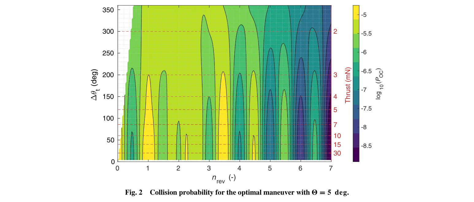
Figure 2 shows the collision probability (logarithmic scale) for the optimal maneuver, as a function of $n_{\text{rev}}$ and $\Delta\theta_t$. Collision probability oscillates with $n_{\text{rev}}$, with local minima located near integer and half-integer values ($n_{\text{rev}} = N + 0.5$), caused by the oscillatory component in the $\zeta$ coordinate. Red dashed lines mark the $\Delta\theta_t = 100^\circ, 200^\circ, 300^\circ$ sections explored in subsequent line plots. The right-side color bar shows the logarithmic collision probability for different thrust levels (2–30 mN), ranging from approximately $10^{-8.5}$ to $10^{-5}$.
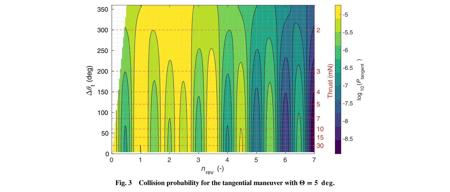
Figure 3 shows the collision probability for pure tangential maneuvers. Using the same coordinate system and color scale as Fig 2, the contour structure is qualitatively very similar to the optimal solution — the oscillation patterns and local minimum locations are nearly identical. This provides initial evidence that over most of the parameter space, the tangential solution is a good approximation to the optimal.
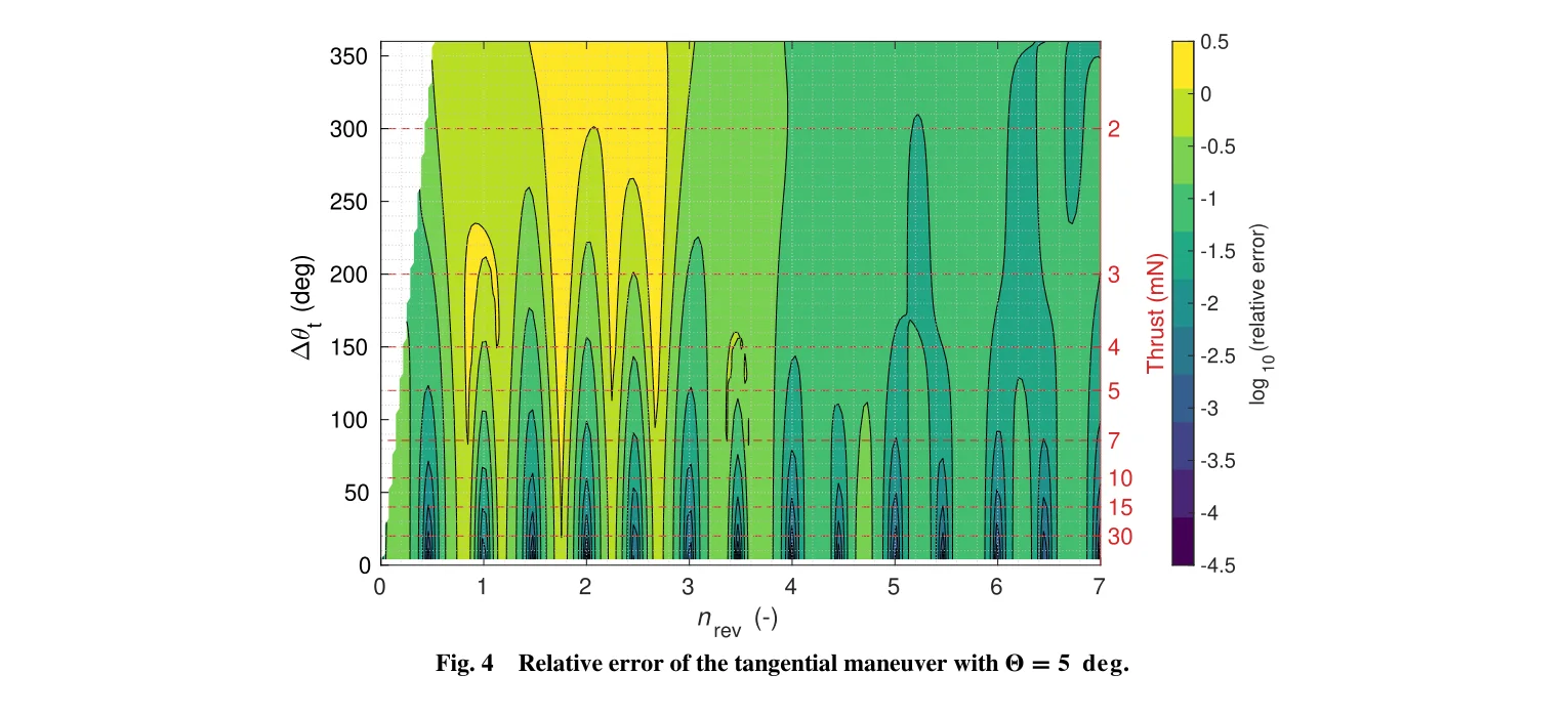
Figure 4 quantifies the relative error of the tangential solution. This is a critical diagnostic: green regions indicate close agreement, while blue/dark regions indicate significant underperformance. Over most of the parameter space (green and yellow regions), the relative error is within $10^{-1}$ (the tangential solution's collision probability is at most a few tens of percent higher than optimal). However, in the region $n_{\text{rev}} \in [0.5, 3]$ with $\Delta\theta_t > 100^\circ$ (blue), the relative error grows substantially — the tangential solution can be worse than optimal by more than an order of magnitude.
7.2 $\Theta = 5^\circ$, $\Delta\theta_t = 200^\circ$: Deep Dive into the Long Arc
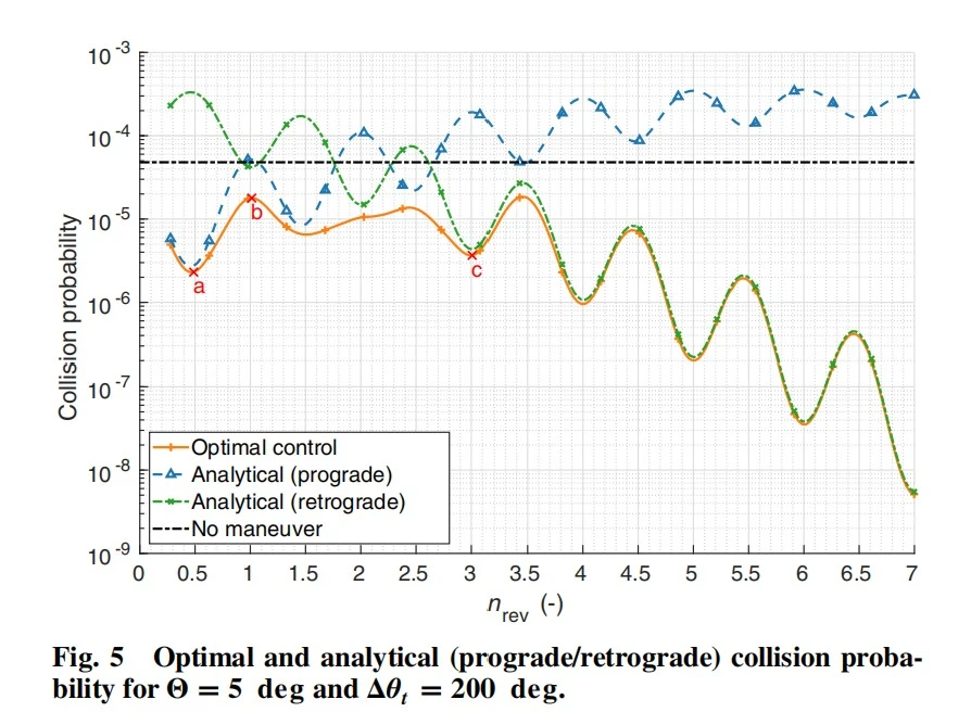
Figure 5 ($\Theta = 5^\circ, \Delta\theta_t = 200^\circ$ section) is the paper's central comparison plot. The blue dashed and green dot-dashed lines correspond to prograde and retrograde tangential solutions, the orange continuous curve traces the optimal solution, and the black dashed line marks the no-maneuver baseline (approximately $4 \times 10^{-5}$). Three characteristic points — a, b, and c — are marked where the optimal-tangential performance gap is most pronounced.
A key observation: over most of the $n_{\text{rev}}$ range, the optimal solution nearly coincides with the retrograde tangential solution — for $\Theta = 5^\circ$, the optimal thrust direction is close to retrograde-tangential at most anticipation times. However, at point a ($n_{\text{rev}} \approx 0.5-1.5$, last-minute maneuver region) and point c ($n_{\text{rev}} \approx 5.5$), the optimal solution significantly outperforms any tangential strategy, reducing collision probability by nearly an order of magnitude.
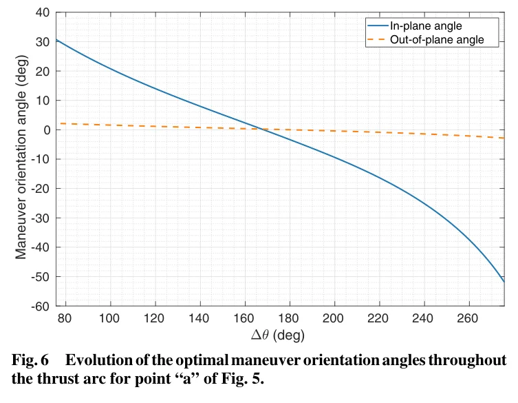
Figure 6 shows the evolution of the in-plane angle $\gamma_{\text{in}}$ (blue) and out-of-plane angle $\gamma_{\text{out}}$ (red) throughout the thrust arc for point a. The horizontal axis is the argument of latitude $\theta$ (from approximately 220° to 460°). At point a (last-minute maneuver), the optimal thrust direction varies dramatically: the in-plane angle transitions smoothly from approximately $-60^\circ$ to $+40^\circ$, while the out-of-plane angle oscillates between $-50^\circ$ and $-10^\circ$. This explains why the tangential solution (fixed direction) performs poorly in this region — the optimal solution requires continuous, large-amplitude steering of the thrust direction.
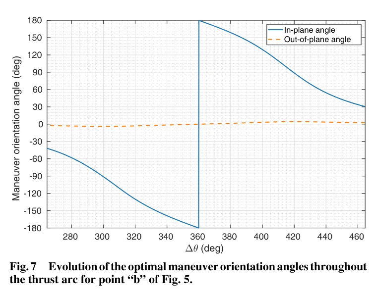
Figure 7 shows the direction evolution at point b. Point b is at $n_{\text{rev}} \approx 2.5$ — the region where optimal and retrograde-tangential solutions nearly coincide. As shown, the in-plane angle (blue) stays near $0^\circ$ and the out-of-plane angle (red) also remains near $0^\circ$ throughout the arc — meaning the optimal thrust direction is essentially pure retrograde-tangential. This is the parameter region where the tangential solution performs best.
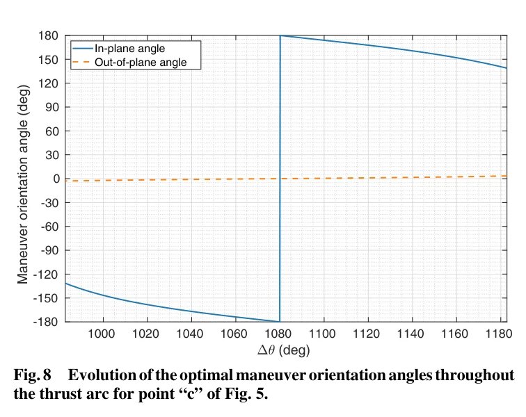
Figure 8 shows the direction evolution at point c. At $n_{\text{rev}} \approx 5.5$ (large anticipation), the in-plane angle (blue) varies substantially (from about $-150^\circ$ to $+30^\circ$), and the out-of-plane angle (red) also fluctuates by about $20^\circ$. This large-amplitude steering again causes the tangential approximation to break down.
7.3 Effect of Thrust Arc Duration: $\Delta\theta_t = 120^\circ, 60^\circ, 30^\circ$
To illustrate how the optimal-tangential gap shrinks with decreasing arc length, the paper presents cross-sections for shorter arcs at $\Theta = 5^\circ$.
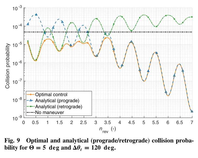
Figure 9 ($\Delta\theta_t = 120^\circ$) shows that when the thrust arc shortens to 120°, the gap between optimal (orange solid) and retrograde-tangential (green dot-dashed) has narrowed considerably compared to Fig 5 ($\Delta\theta_t = 200^\circ$). Over most of the $n_{\text{rev}}$ range, the two are nearly indistinguishable. The overall collision probability level has also risen (approximately $10^{-8}$ to $10^{-3}$), as shorter thrust arcs produce smaller b-plane displacements.
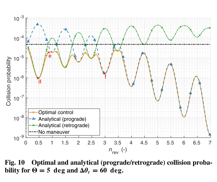
Figure 10 ($\Delta\theta_t = 60^\circ$) further reinforces this trend. Three new characteristic points — d, e, f — are marked. The optimal and retrograde-tangential solutions are nearly coincident across almost the entire $n_{\text{rev}}$ range — only near point d ($n_{\text{rev}} \approx 0.5$, last-minute) does the optimal solution show a modest advantage. This indicates that for shorter thrust arcs, the tangential solution is virtually equivalent to the optimal.
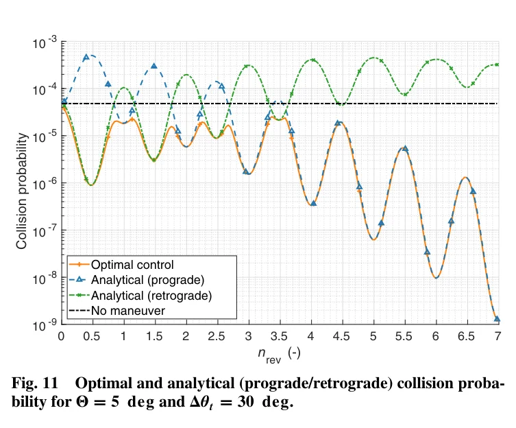
Figure 11 ($\Delta\theta_t = 30^\circ$) is the limiting case of this sequence. At a 30° short arc, the optimal, prograde-tangential and retrograde-tangential curves have converged almost perfectly — the low-thrust solution now transitions smoothly to the impulsive solution of Bombardelli & Hernando-Ayuso (2015). The collision probability variation with $n_{\text{rev}}$ is also smoother, with reduced oscillation amplitude.
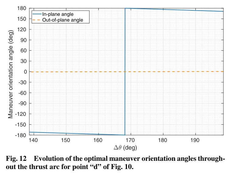
Figure 12 shows the direction evolution at point d. Compared to point a (200° arc, Fig 6), the variation amplitudes of both the in-plane angle (blue) and out-of-plane angle (red) are substantially reduced — the in-plane angle varies within a narrow band of approximately $-140^\circ$ to $-110^\circ$, while the out-of-plane angle remains nearly constant at about $20^\circ$. This reflects the tendency for short-arc optimal thrust directions to approach a constant.
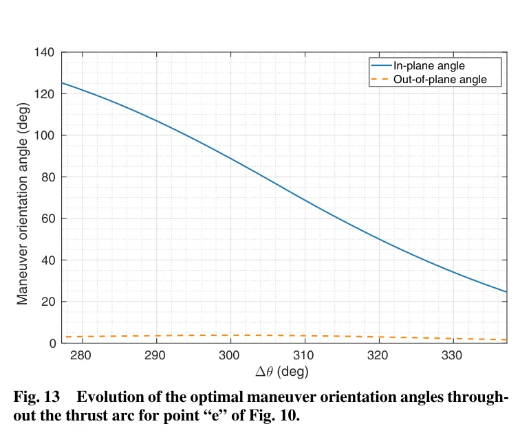
Figure 13 shows the direction evolution at point e. Located near $n_{\text{rev}} \approx 2$, the in-plane angle (blue) varies between $0^\circ$ and $120^\circ$, while the out-of-plane angle (red) stays near $4^\circ$ — the thrust remains predominantly in the orbital plane, close to tangential.
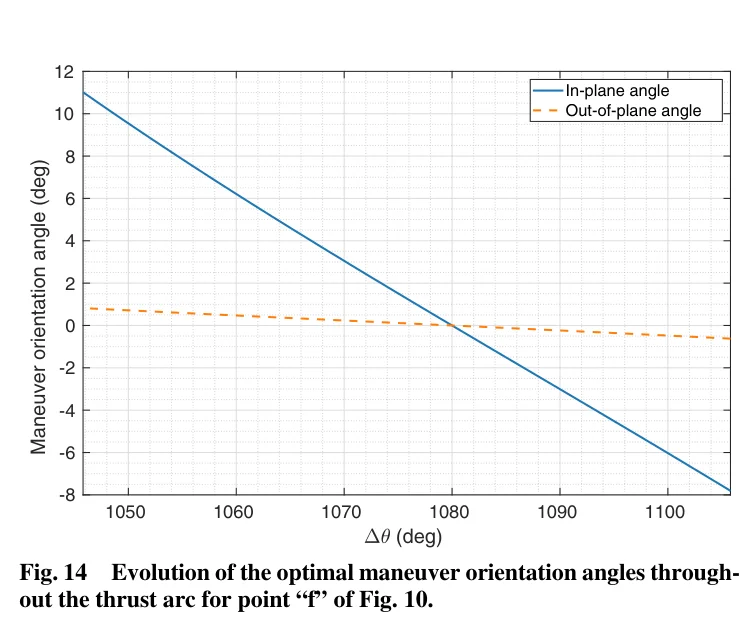
Figure 14 shows the direction evolution at point f. Near $n_{\text{rev}} \approx 3.5$, the thrust again remains essentially in-plane (out-of-plane angle near 0°), with the in-plane angle (blue) exhibiting only minor fluctuations between $-6^\circ$ and $+12^\circ$. This further corroborates the validity of the tangential approximation in this parameter regime.
7.4 The $\Theta = 0^\circ$ Case: Covariance Ellipse Aligned with b-Plane
When the covariance ellipse principal axes align perfectly with the b-plane coordinate axes ($\Theta = 0^\circ$), the encounter geometry takes on special properties.
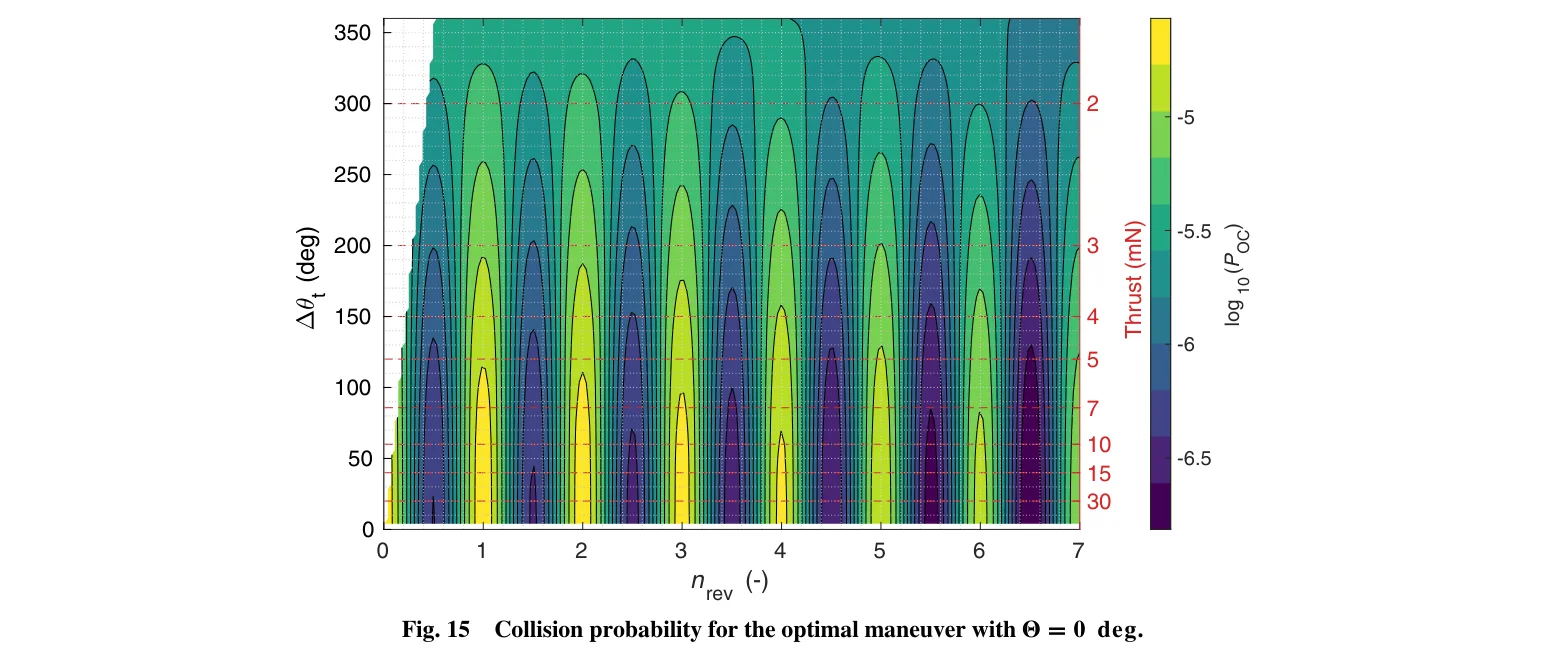
Figure 15 shows the optimal collision probability for $\Theta = 0^\circ$. Compared to $\Theta = 5^\circ$ (Fig 2), a striking difference emerges: the oscillation pattern in $n_{\text{rev}}$ is more regular — local minima line up neatly at $n_{\text{rev}} = N + 0.5$ — and the overall probability level is lower (most regions between $10^{-6}$ and $10^{-5}$), indicating that the $\Theta = 0^\circ$ covariance configuration is more favorable for collision avoidance.
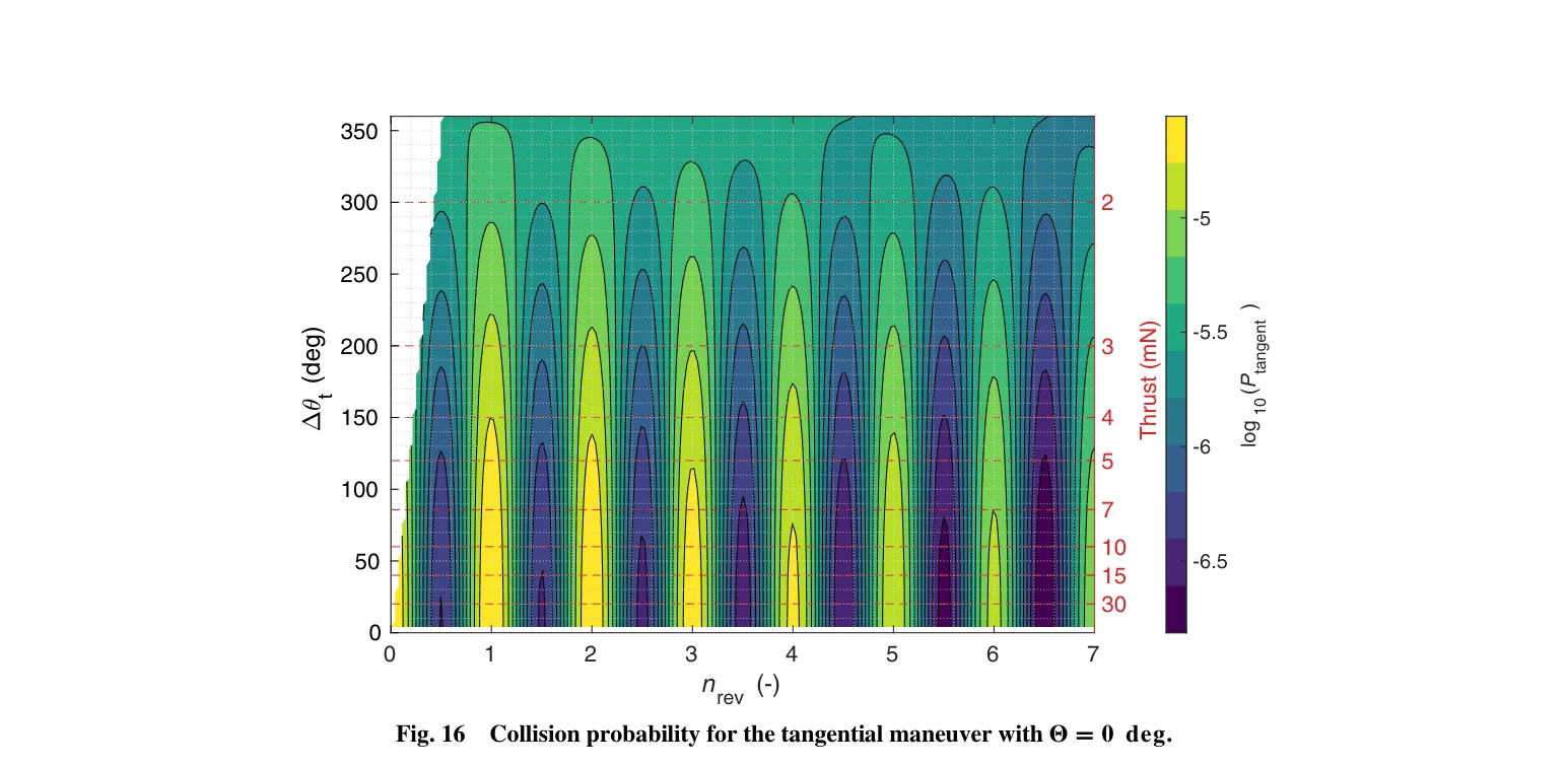
Figure 16 shows the tangential collision probability for $\Theta = 0^\circ$. Compared with Fig 15, the tangential contour structure is almost perfectly identical to the optimal — a fact that will be confirmed quantitatively in Fig 17.
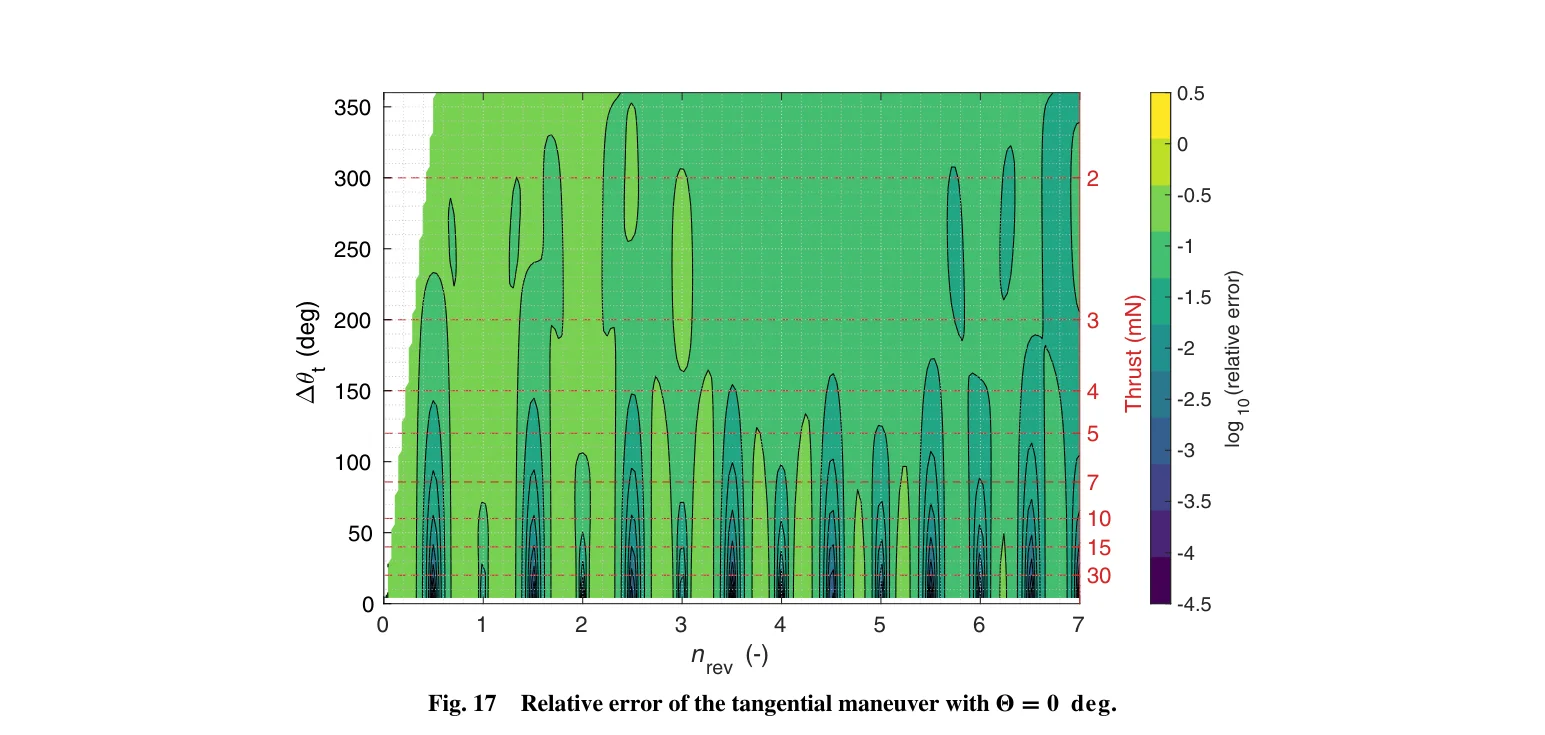
Figure 17 is the most important diagnostic for the $\Theta = 0^\circ$ case. The logarithmic relative error lies almost entirely between $-0.5$ and $0.5$ (corresponding to a relative error between about $0.3\times$ and $3\times$), with large swaths of the parameter space showing essentially zero error (white/light regions). This means that when $\Theta = 0^\circ$, the tangential solution is virtually indistinguishable from the optimal — in engineering practice, one can use the analytical tangential formulas directly without running any numerical optimization.
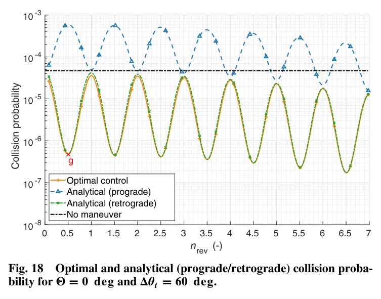
Figure 18 ($\Theta = 0^\circ, \Delta\theta_t = 60^\circ$ section) provides line-plot confirmation. The optimal (orange solid) and retrograde-tangential (green dot-dashed) curves are perfectly coincident across the entire $n_{\text{rev}}$ range. Point g is marked; its direction evolution is shown below.
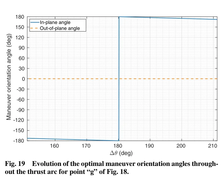
Figure 19 shows the direction evolution at point g. The in-plane angle (blue) sweeps through nearly the full 360° range (from $-150^\circ$ to $+180^\circ$), but critically, the out-of-plane angle (red) remains pinned at $0^\circ$ throughout. This means that at $\Theta = 0^\circ$, the optimal thrust lies entirely in the orbital plane — no out-of-plane component is needed. Although the thrust direction varies with time, its effect is equivalent to tangential thrust.
7.5 The $\Theta = -5^\circ$ Case: Covariance Ellipse Tilted Oppositely
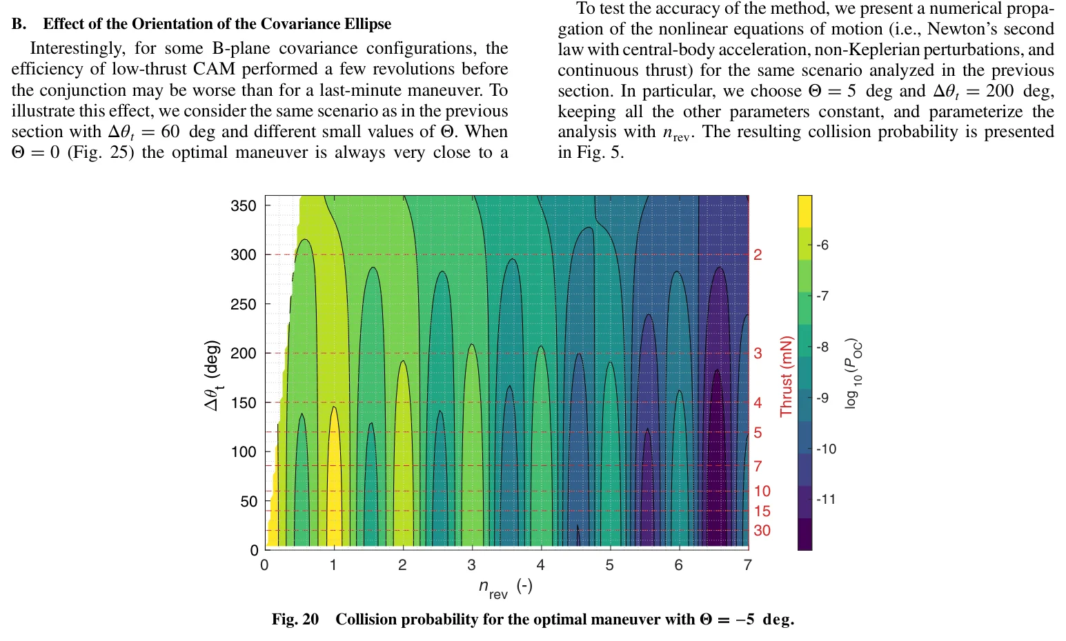
Figure 20 shows the optimal collision probability for $\Theta = -5^\circ$. Compared to $\Theta = +5^\circ$ (Fig 2), the collision probability is dramatically lower — most regions lie between $10^{-11}$ and $10^{-6}$, 2–3 orders of magnitude below the $\Theta = +5^\circ$ case. The oscillation pattern is also more regular, with neatly aligned local minima. This reveals an important phenomenon: when the covariance ellipse tilts in the negative direction, the secular component of tangential thrust (increasing miss distance along $\xi$) moves the b-vector along the low-probability direction of the covariance ellipse, dramatically boosting avoidance efficiency.
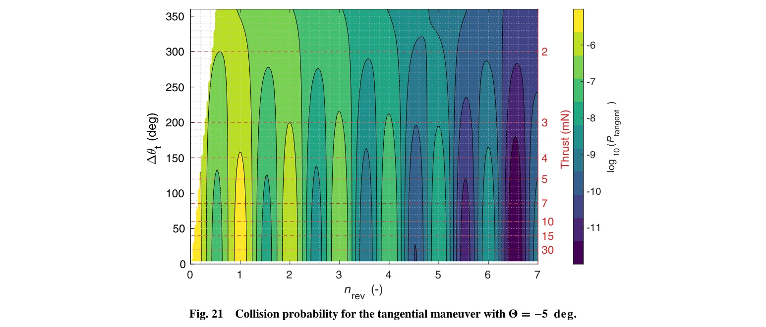
Figure 21 shows the tangential collision probability for $\Theta = -5^\circ$. Comparing with Fig 20, the tangential solution still captures the overall structure of the optimal very well — probability levels, oscillation patterns, and local minimum locations are all highly consistent.
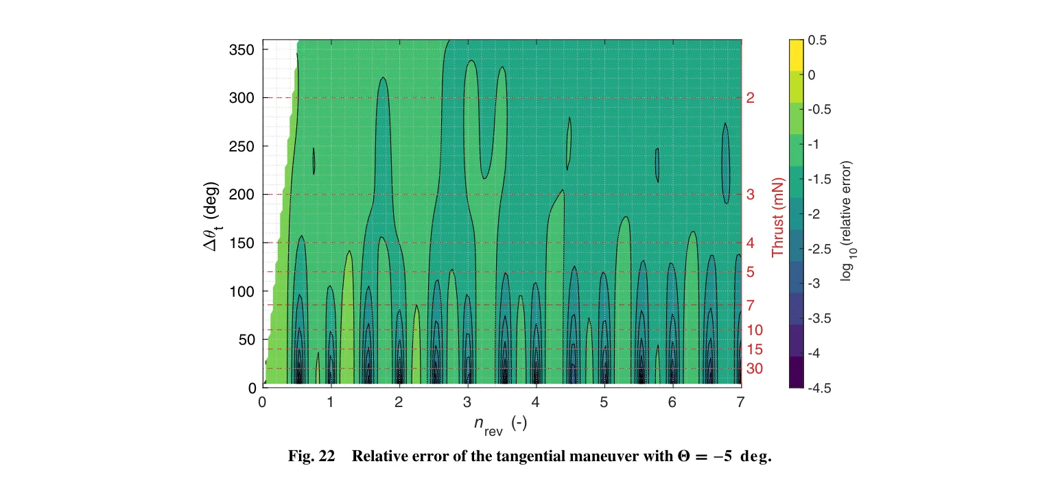
Figure 22 quantifies the relative error of the tangential solution at $\Theta = -5^\circ$. Compared to $\Theta = 0^\circ$ (Fig 17), the error is somewhat larger — in the region $n_{\text{rev}} \in [0.5, 2]$ with $\Delta\theta_t > 150^\circ$, the relative error can reach approximately 1–3. Nevertheless, overall the tangential solution still provides a good approximation, especially at large $n_{\text{rev}}$ and small $\Delta\theta_t$.
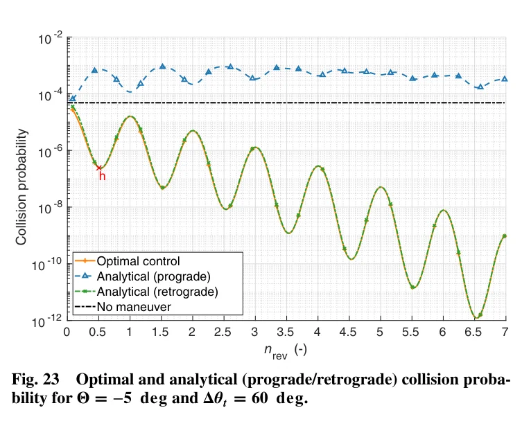
Figure 23 ($\Theta = -5^\circ, \Delta\theta_t = 60^\circ$ section) shows that for a short arc, the optimal (orange solid) and retrograde-tangential (green dot-dashed) are nearly indistinguishable. Compared to the $\Theta = +5^\circ$ counterpart (Fig 10), the collision probability is approximately 4 orders of magnitude lower — once again highlighting the decisive influence of covariance ellipse orientation on avoidance efficiency. Point h is marked.
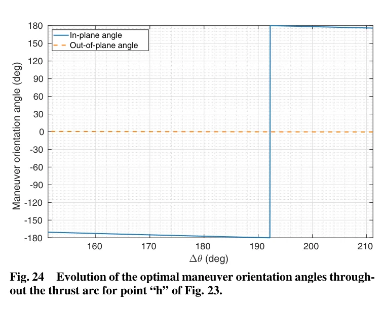
Figure 24 shows the direction evolution at point h. The in-plane angle (blue) varies between approximately $-150^\circ$ and $+180^\circ$, but the out-of-plane angle (red) remains near $0^\circ$ — similar to the $\Theta = 0^\circ$ case, the optimal thrust is essentially confined to the orbital plane.
7.6 Extended Anticipation Analysis: $\Theta = 0^\circ, 1^\circ, 3^\circ, 5^\circ$
To study the influence of covariance ellipse orientation over a larger $n_{\text{rev}}$ range, the analysis is extended to $n_{\text{rev}} \in [0, 14]$.
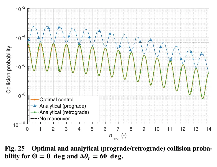
Figure 25 ($\Theta = 0^\circ$, extended to $n_{\text{rev}} = 14$) shows the collision probability continuing to oscillate and decline beyond $n_{\text{rev}} = 7$, reaching as low as approximately $10^{-8}$. The optimal, prograde-tangential, and retrograde-tangential curves remain perfectly coincident throughout, further confirming that at $\Theta = 0^\circ$, tangential = optimal.
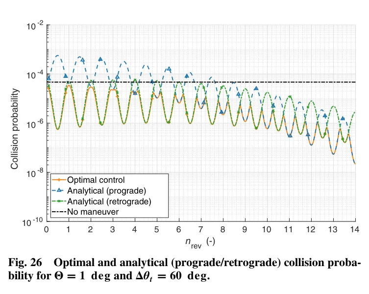
Figure 26 ($\Theta = 1^\circ$) is one of the paper's most revealing plots. A mere $1^\circ$ tilt of the covariance ellipse produces discernible differences between optimal (orange) and tangential solutions: in the range $n_{\text{rev}} \in [5, 9]$, the tangential local minima vanish or shift, while the optimal continues to maintain lower collision probability. At large $n_{\text{rev}}$ (>10), the tangential collision probability can exceed the optimal by up to two orders of magnitude. This demonstrates that even the smallest covariance ellipse tilt significantly impacts maneuver strategy selection at long anticipation times.
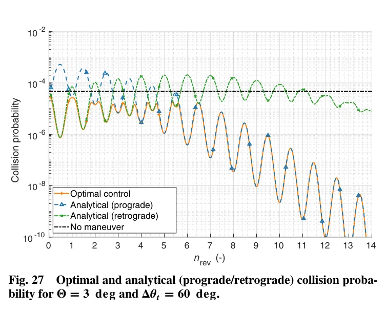
Figure 27 ($\Theta = 3^\circ$) amplifies the trends observed at $\Theta = 1^\circ$. The gap between optimal and tangential solutions is more pronounced: at large $n_{\text{rev}}$, the tangential solution nearly fails entirely, while the optimal still maintains collision probability below $10^{-6}$.
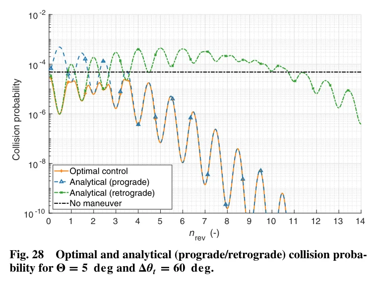
Figure 28 ($\Theta = 5^\circ$, extended to $n_{\text{rev}} = 14$) shows the largest tilt case. At large $n_{\text{rev}}$ (>10), the tangential collision probability ceases to decline and may even rebound, while the optimal solution continues its descent. This clearly demonstrates that the covariance ellipse orientation $\Theta$ is the key parameter determining the effectiveness of long-anticipation maneuver strategies, and a tilt as small as $1^\circ$ suffices to alter the nature of the optimal strategy.
7.7 B-Plane Trajectory Visualization: Understanding Tangential vs. Optimal
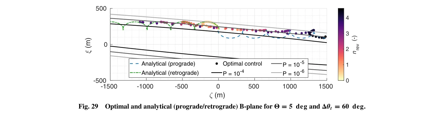
Figure 29 is the key visualization for understanding the fundamental difference between tangential and optimal solutions. It plots three trajectories simultaneously in the $\xi$-$\zeta$ plane:
- Blue dashed line: prograde-tangential b-plane trajectory
- Green dashed line: retrograde-tangential b-plane trajectory
- Colored scatter points: optimal b-plane trajectory (color represents $n_{\text{rev}}$, from yellow (0 revs) to deep purple (~4.5 revs))
The background diagonal lines are constant collision probability contours ($P = 10^{-4}, 10^{-5}, 10^{-6}$), whose orientation is determined by the covariance ellipse tilt $\Theta = 5^\circ$.
Key insight:
- Retrograde maneuvers (green) perform better at short anticipation (low $n_{\text{rev}}$) — their trajectory achieves large displacement in the $+\xi$ direction, moving along the decreasing-probability contour direction
- Prograde maneuvers (blue) perform better at long anticipation (high $n_{\text{rev}}$) — their $\zeta$ variation aligns with the covariance ellipse tilt direction
- The optimal solution (colored points) switches between the two: biased toward retrograde at low $n_{\text{rev}}$, toward prograde at high $n_{\text{rev}}$
This plot provides an intuitive explanation for why, when $\Theta > 0^\circ$, the optimal strategy is not simply "maneuver as early as possible" — rather, across different $n_{\text{rev}}$ intervals, the optimal thrust direction must align with the tilted probability contours of the covariance ellipse.
8. Accuracy Validation: Analytical/Semi-Analytical vs. High-Fidelity Propagation
The paper rigorously validates the analytical/semi-analytical methods through high-fidelity numerical propagation (EGM96 gravity model truncated to degree and order 50, including lunar, solar, and planetary gravity).
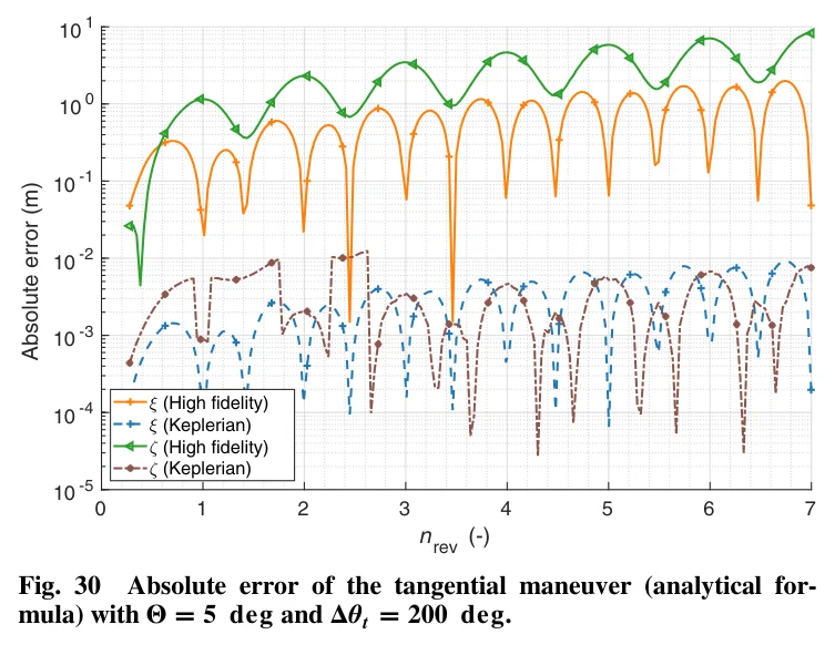
Figure 30 shows the absolute error of the tangential analytical formula. Four curves correspond to $\xi$ and $\zeta$ coordinates under Keplerian and high-fidelity force models. In the Keplerian case, the absolute error is on the order of $10^{-4}$ m — essentially negligible. Under the high-fidelity model, absolute error increases to approximately $10^{-1}$ to $10^0$ m (decimeter to meter level), but against the backdrop of LEO encounter distances typically in the hundreds of meters to kilometers, this is entirely acceptable. The $\xi$ error (blue/green) is slightly larger than the $\zeta$ error (red/orange), consistent with the $\xi$ coordinate containing a secular term with greater cumulative effect.
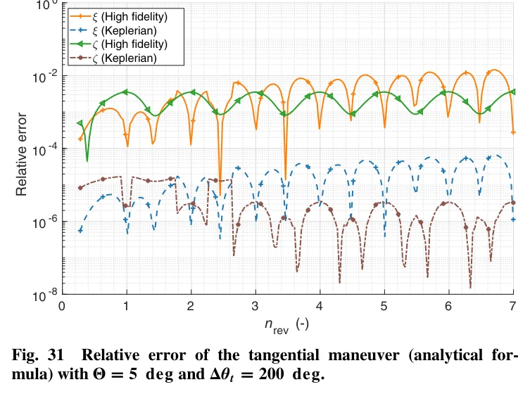
Figure 31 shows the relative error of the tangential analytical formula. Under the Keplerian model, relative error ranges from $10^{-6}$ to $10^{-2}$. Under the high-fidelity model, relative error is approximately $10^{-2}$ to $10^0$ (1% to 100%) — near the $\zeta \to 0$ singularity, relative error is large, but the absolute error itself is small, so it has no practical impact on collision probability computation.
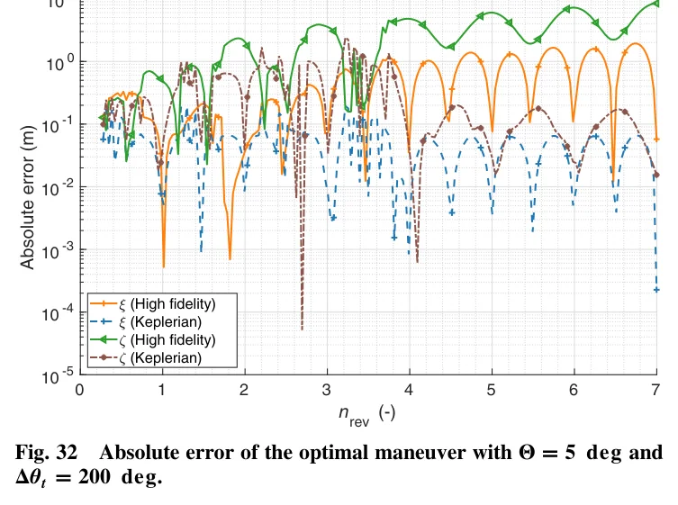
Figure 32 shows the absolute error of the optimal control solution. Compared to Fig 30 (tangential), the optimal solution's absolute error under the high-fidelity model is somewhat larger — approximately $10^0$ to $10^1$ m (meter to decameter level). This is because the optimal control solution involves repeated operations on the $\mathbf{M}_0$ matrix, and numerical errors are slightly amplified by the iterative TPBVP solver. Even so, errors at the 10 m level remain acceptable for operational purposes.
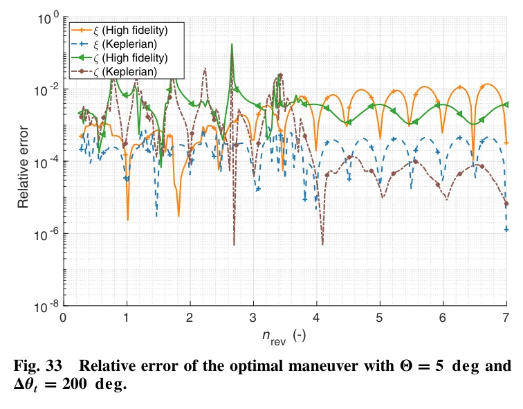
Figure 33 shows the relative error of the optimal control solution. The pattern is similar to Fig 31 (tangential): negligible error in the Keplerian case, relative error approximately $10^{-2}$ to $10^0$ under the high-fidelity model. The $\zeta$ coordinate exhibits larger relative error near the singularity, but absolute error remains acceptable.
Overall accuracy conclusions:
- Keplerian case: absolute error in b-plane coordinates under 0.01 m, relative error negligible
- Perturbed case (LEO): absolute error under 10 m, relative error approximately 1% — consistent with the impulsive paper [Bombardelli & Hernando-Ayuso, 2015]
- J2 and other environmental perturbations have negligible impact on b-plane predictions for operational purposes
9. Conclusions and Implications
Hernando-Ayuso & Bombardelli (2021) successfully extend the optimal control theory of collision avoidance from the impulsive domain to the low-thrust domain. Their key contributions can be summarized as:
-
Continuity and unification of methods — The paper uses the same b-plane framework and thrust direction parameterization as the impulsive work, ensuring seamless theoretical and practical integration between the two domains
-
Elegant marriage of analytical and numerical approaches — Pontryagin's maximum principle reduces the infinite-dimensional optimal control problem to a 2D TPBVP, while a fully analytical solution is provided for the tangential thrust case, enabling sub-millisecond rapid assessment
-
Engineering practicality of the tangential solution — Over most of the parameter space (especially at $\Theta = 0^\circ$ and near optimal phasing), the tangential solution performs nearly as well as the optimal control, providing a rapid assessment tool that requires no optimization
-
Pivotal role of covariance orientation — The paper reveals a counterintuitive phenomenon: a mere $1^\circ$ tilt of the covariance ellipse can reverse the conclusion of "maneuver early" vs. "maneuver late," directly impacting constellation operations strategy
-
Accuracy sufficient for engineering needs — Errors under high-fidelity force models remain within 10 m (absolute) and 1% (relative), validating the engineering applicability of b-plane linear theory
Implications for engineering practice:
Six years before this paper, Bombardelli & Hernando-Ayuso (2015) transformed impulsive collision avoidance from "numerical scanning" to "analytical solving." Now, Hernando-Ayuso & Bombardelli (2021) extend this paradigm into the low-thrust era. With tens of thousands of electrically propelled constellation satellites being deployed, the methodology presented in this paper will become a core tool for collision avoidance operations.
If the first paper answered "in which direction should I fire a single impulse to be most effective?", this paper answers "how should I continuously steer my thrust direction throughout a finite thrust arc to minimize collision probability?" — the former is an algebraic problem, the latter a control problem. Together, they form the complete picture of modern collision avoidance theory.
References
-
Bombardelli, C., and Hernando-Ayuso, J., "Optimal Impulsive Collision Avoidance in Low Earth Orbit", J. Guidance, Control, and Dynamics, Vol. 38, No. 2, 2015, pp. 217–225. DOI: 10.2514/1.G000742
-
Hernando-Ayuso, J., and Bombardelli, C., "Low-Thrust Collision Avoidance in Circular Orbits", J. Guidance, Control, and Dynamics, Vol. 44, No. 5, 2021, pp. 984–995. DOI: 10.2514/1.G005547
-
Bombardelli, C., Baù, G., and Peláez, J., "Asymptotic Solution for the Two-Body Problem with Constant Tangential Thrust Acceleration", Celestial Mechanics and Dynamical Astronomy, Vol. 110, No. 3, 2011, pp. 239–256.
-
Bombardelli, C., "Analytical Formulation of Impulsive Collision Avoidance Dynamics", Celestial Mechanics and Dynamical Astronomy, Vol. 118, No. 2, 2014, pp. 99–114.
-
Chan, F. K., Spacecraft Collision Probability, Aerospace Press, El Segundo, CA, 2008.
-
Salemme, G., Armellin, R., and Di Lizia, P., "Continuous-Thrust Collision Avoidance Manoeuvres Optimization", AIAA SciTech 2020 Forum, AIAA Paper 2020-0231.
-
Bryson, A. E., and Ho, Y.-C., Applied Optimal Control, Taylor & Francis, 1975.
-
García-Pelayo, R., and Hernando-Ayuso, J., "Series for Collision Probability in Short-Encounter Model", J. Guidance, Control, and Dynamics, Vol. 39, No. 8, 2016, pp. 1908–1916.