[Classic Paper Review] Attention Is All You Need — The Transformer Explained
2026-06-28
Attention Is All You Need — The Transformer Explained
Paper: Ashish Vaswani, Noam Shazeer, Niki Parmar, Jakob Uszkoreit, Llion Jones, Aidan N. Gomez, Łukasz Kaiser, Illia Polosukhin. "Attention Is All You Need." Advances in Neural Information Processing Systems 30 (NIPS 2017).
Affiliations: Google Brain, Google Research, University of Toronto
1. Introduction: Why Do We Need the Transformer?
Before 2017, the dominant approaches to sequence modeling and machine translation were encoder-decoder architectures built on recurrent neural networks (RNNs), specifically Long Short-Term Memory (LSTM) networks and Gated Recurrent Units (GRUs). These models encode an input sequence step-by-step into a hidden state vector, from which the decoder generates the output sequence one token at a time.
RNNs, however, suffer from a fundamental limitation: the inherently sequential nature of their computation. At time step $t$, the hidden state $h_t$ is a function of the previous hidden state $h_{t-1}$ and the current input $x_t$:
$$h_t = f(h_{t-1}, x_t)$$
This recurrence means that computation cannot be parallelized across sequence positions — before processing the 100th token, the model must first process the preceding 99 tokens. As sequences grow longer, this not only slows training dramatically (memory constraints limit batching across examples) but also forces long-range dependencies to propagate through many time steps, making the model vulnerable to vanishing or exploding gradients.
Attention mechanisms had already been incorporated into sequence models prior to this work. Bahdanau et al. (2014) augmented RNN encoder-decoders with attention, allowing the decoder to attend over all encoder positions when generating each output token, rather than relying solely on the final hidden state. But the critical point is this: attention was always used as an auxiliary component on top of an RNN. The core computational structure remained recurrent.
Vaswani et al. posed a simple yet daring question in their 2017 paper: What if we dispense with recurrence and convolution entirely, and build the entire model using only attention mechanisms? The answer is the Transformer — the first sequence transduction model based solely on attention.
The Transformer offers three key advantages:
- Massively parallelizable: Computation at each position does not depend on the output of previous positions (except for the autoregressive constraint in the decoder), enabling dramatic training speedups.
- Constant path length: Information between any two input or output positions requires only a constant number of operations ($O(1)$), compared to $O(n)$ for RNNs.
- Shorter training time: On the WMT 2014 English-German translation task, the Transformer trained for just 12 hours on 8 P100 GPUs and reached 28.4 BLEU — outperforming the best existing ensemble models by over 2 BLEU points.
2. Background: Why Can Attention Replace Recurrence and Convolution?
Prior to the Transformer, several efforts had already targeted the goal of reducing sequential computation. ByteNet and ConvS2S, for instance, used convolutional neural networks as their basic building block, computing hidden representations in parallel for all input and output positions. However, these models share a common drawback: the number of operations required to relate signals from two arbitrary positions grows with the distance between them — linearly for ConvS2S ($O(n)$) and logarithmically for ByteNet ($O(\log n)$). This makes learning long-range dependencies increasingly difficult.
The Transformer reduces this to a constant $O(1)$. There is, however, a trade-off: because the attention mechanism computes a weighted average over all input positions, the effective resolution is reduced. The paper compensates for this through Multi-Head Attention, which allows the model to jointly attend to information from different representation subspaces.
Self-attention had already been successfully applied to tasks including reading comprehension, abstractive summarization, and textual entailment before the Transformer. But all prior work used self-attention in conjunction with an RNN. The Transformer is the first model to rely entirely on self-attention.
3. Model Architecture: A Layer-by-Layer Breakdown
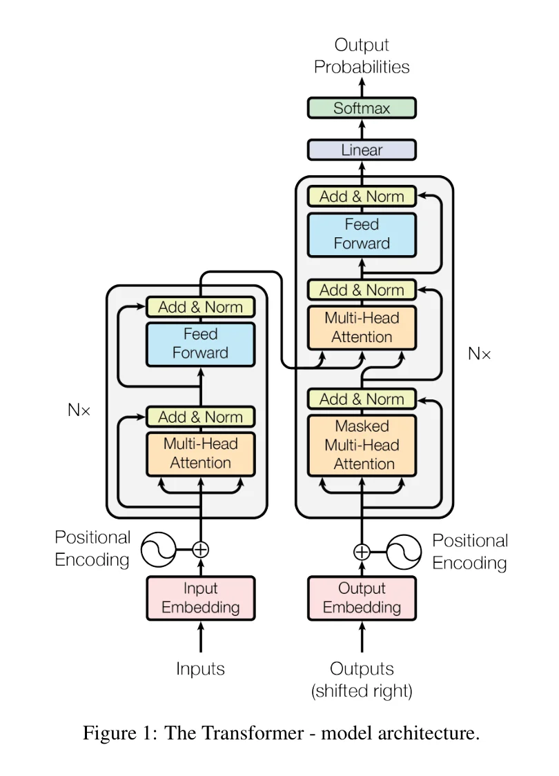
Figure 1 shows the complete Transformer architecture. At a glance, it consists of an Encoder on the left and a Decoder on the right — a classic sequence-to-sequence (Seq2Seq) structure.
3.1 Encoder and Decoder Stacks
The Encoder is composed of a stack of $N = 6$ identical layers. Each layer has two sub-layers:
- A Multi-Head Self-Attention sub-layer
- A Position-wise Fully Connected Feed-Forward Network sub-layer
The output of each sub-layer is wrapped with a residual connection followed by layer normalization:
$$\text{Output} = \text{LayerNorm}(x + \text{Sublayer}(x))$$
To facilitate these residual connections, all sub-layers in the model, as well as the embedding layers, produce outputs of dimension $d_{\text{model}} = 512$.
The Decoder is also composed of a stack of $N = 6$ identical layers. In addition to the two sub-layers found in each encoder layer, the decoder inserts a third sub-layer that performs Multi-Head Attention over the output of the encoder stack — this is the classic Encoder-Decoder Attention. As with the encoder, residual connections and layer normalization follow each sub-layer.
Crucially, the decoder's self-attention sub-layer is modified: masking prevents position $i$ from attending to any position $j > i$. This is implemented by setting the corresponding values in the Softmax input to $-\infty$. Combined with the fact that the output embeddings are offset by one position, this ensures that the prediction for position $i$ can depend only on known outputs at positions less than $i$, preserving the autoregressive property.
3.2 Attention: The Heart of the Model
An attention function can be described as mapping a Query and a set of Key-Value pairs to an output. The output is a weighted sum of the values, where the weight assigned to each value is computed by a compatibility function of the query with the corresponding key.
3.2.1 Scaled Dot-Product Attention
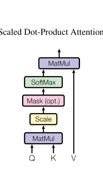
As shown in Figure 2 (left), the Scaled Dot-Product Attention proceeds as follows:
- Compute the dot products of the query $Q$ with all keys $K$: $QK^T$
- Scale the dot products by dividing by $\sqrt{d_k}$, where $d_k$ is the dimension of the key vectors
- Apply a Softmax function to obtain the weight distribution
- Multiply the weights by the values $V$ to produce the output
The mathematical expression is:
$$\text{Attention}(Q, K, V) = \text{softmax}\left(\frac{QK^T}{\sqrt{d_k}}\right)V \tag{1}$$
In practice, we pack a set of queries into matrix $Q$, and keys and values into matrices $K$ and $V$. This matrix formulation allows the computation to leverage highly optimized linear algebra libraries for exceptional speed and memory efficiency.
Why divide by $\sqrt{d_k}$? This is a critical detail in the paper. There are two common forms of attention: additive attention and dot-product attention. While the two are similar in theoretical complexity, dot-product attention is much faster and more space-efficient in practice because it can be implemented using matrix multiplication.
However, for large values of $d_k$, the dot products grow large in magnitude, pushing the Softmax function into regions where it has extremely small gradients. The paper's reasoning: assume the components of $q$ and $k$ are independent random variables with mean 0 and variance 1. Then the dot product $q \cdot k = \sum_i q_i k_i$ has mean 0 and variance $d_k$. By dividing by $\sqrt{d_k}$, the variance is normalized back to 1, keeping the Softmax input in a well-behaved range and preserving gradient flow.
3.2.2 Multi-Head Attention
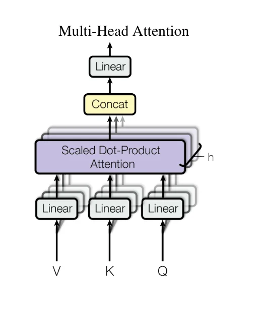
Rather than performing a single attention function with $d_{\text{model}}$-dimensional keys, values, and queries, the authors found it beneficial to linearly project the queries, keys, and values $h$ times with different learned projections. Specifically:
- $h = 8$ parallel attention heads
- Each head operates at reduced dimensionality: $d_k = d_v = d_{\text{model}} / h = 512 / 8 = 64$
Each head computes:
$$\text{head}_i = \text{Attention}(QW_i^Q, KW_i^K, VW_i^V)$$
where $W_i^Q \in \mathbb{R}^{d_{\text{model}} \times d_k}$, $W_i^K \in \mathbb{R}^{d_{\text{model}} \times d_k}$, $W_i^V \in \mathbb{R}^{d_{\text{model}} \times d_v}$ are the projection matrices. The outputs of all heads are concatenated and then projected once more:
$$\text{MultiHead}(Q, K, V) = \text{Concat}(\text{head}_1, ..., \text{head}_h) W^O$$
where $W^O \in \mathbb{R}^{h d_v \times d_{\text{model}}}$.
Why multiple heads? A single attention head can only attend from one "perspective" — it assigns a fixed set of weights to each position based on one compatibility function. Different heads can learn to attend to different types of relationships: some may focus on syntactic structure (e.g., subject-verb relationships), others on semantic relevance, and still others on positional proximity. By running $h$ heads in parallel, the model can jointly capture diverse dependencies from different representation subspaces simultaneously.
Because each head operates at reduced dimensionality (from 512 down to 64), the total computational cost of $h$ heads is similar to that of single-head attention with full dimensionality. This is an elegant design: the same computational budget buys significantly richer representational capacity.
3.2.3 Three Applications of Attention in the Transformer
The Transformer employs multi-head attention in three distinct ways:
-
Encoder-Decoder Attention: The queries come from the previous decoder layer, while the keys and values come from the output of the encoder. This allows every position in the decoder to attend over all positions in the input sequence, mimicking the classic attention mechanism in Seq2Seq models.
-
Encoder Self-Attention: All keys, values, and queries come from the same place — the output of the previous layer in the encoder. Each position in the encoder can attend to all positions in the previous encoder layer.
-
Decoder Masked Self-Attention: Similar to encoder self-attention, but masking prevents position $i$ from attending to position $j > i$. In practice, we set all values in the Softmax input corresponding to illegal connections to $-\infty$, so their Softmax weights become zero. This preserves the autoregressive property essential for generation.
3.3 Position-wise Feed-Forward Networks
In addition to the attention sub-layers, each layer in the encoder and decoder contains a fully connected feed-forward network, applied to each position separately and identically. It consists of two linear transformations with a ReLU activation in between:
$$\text{FFN}(x) = \max(0, xW_1 + b_1)W_2 + b_2$$
The inner dimension is $d_{ff} = 2048$. In other words, the first linear layer expands the dimension from 512 to 2048, and the second projects it back down to 512.
This can be understood as two $1 \times 1$ convolutions (since each position is processed independently), or as a per-position nonlinear transformation applied after the attention mechanism has aggregated contextual information — further enhancing the representational capacity at each position.
3.4 Embeddings and Softmax
Like other sequence transduction models, the Transformer uses learned embeddings to convert input and output tokens into vectors of dimension $d_{\text{model}}$. At the decoder output, a linear transformation followed by a Softmax function converts the decoder output into predicted next-token probabilities.
The paper also employs a common technique: weight tying between the input embedding layer and the pre-Softmax linear transformation. Additionally, the embedding outputs are multiplied by $\sqrt{d_{\text{model}}}$ to prevent the embedding values from being too small relative to the positional encodings.
3.5 Positional Encoding
Since the Transformer contains no recurrence and no convolution, the model has no inherent notion of sequence order. To inject information about token positions, the paper adds Positional Encodings to the input embeddings at the bottoms of both the encoder and decoder stacks.
The positional encodings have the same dimension $d_{\text{model}}$ as the embeddings, so they can be summed directly. The paper uses sine and cosine functions of different frequencies:
$$ PE_{(pos, 2i)} = \sin\left(\frac{pos}{10000^{2i / d_{\text{model}}}}\right) $$
$$ PE_{(pos, 2i+1)} = \cos\left(\frac{pos}{10000^{2i / d_{\text{model}}}}\right) $$
where $pos$ is the position and $i$ is the dimension index. Each dimension of the positional encoding corresponds to a sinusoid with a wavelength that forms a geometric progression from $2\pi$ to $10000 \cdot 2\pi$.
Why sine and cosine? The paper hypothesizes that this encoding would allow the model to easily learn to attend by relative positions, since for any fixed offset $k$, $PE_{pos+k}$ can be represented as a linear function of $PE_{pos}$ — a consequence of the addition formulas for sine and cosine.
Moreover, the sinusoidal encoding offers an additional advantage: it may allow the model to extrapolate to sequence lengths longer than those encountered during training, since the sinusoids are defined for any position value. Learned positional embeddings cannot do this. The ablation study (Table 3, row (E)) confirms that learned positional embeddings and sinusoidal encodings produce nearly identical results, validating the choice of the more flexible sinusoidal approach.
4. Why Self-Attention?
Section 4 of the paper systematically compares self-attention layers to recurrent and convolutional layers along three dimensions:
| Layer Type | Complexity per Layer | Sequential Operations | Maximum Path Length |
|---|---|---|---|
| Self-Attention | $O(n^2 \cdot d)$ | $O(1)$ | $O(1)$ |
| Recurrent | $O(n \cdot d^2)$ | $O(n)$ | $O(n)$ |
| Convolutional | $O(k \cdot n \cdot d^2)$ | $O(1)$ | $O(\log_k(n))$ |
| Self-Attention (restricted) | $O(r \cdot n \cdot d)$ | $O(1)$ | $O(n/r)$ |
This table (Table 1 in the paper) reveals several key advantages of self-attention:
-
Parallelization (Sequential Operations): Self-attention requires only $O(1)$ sequential operations — all positions can be computed simultaneously. RNNs require $O(n)$ sequential steps, making full parallelization impossible.
-
Maximum Path Length: This measures the longest path that forward and backward signals must traverse through the network. For self-attention, it is $O(1)$ — information between any two positions flows through a single attention operation. For RNNs, it is $O(n)$, requiring step-by-step propagation. This directly affects the model's ability to learn long-range dependencies.
-
Computational Complexity: When the sequence length $n$ is smaller than the representation dimension $d$ (in machine translation, $n$ is typically tens to hundreds, while $d = 512$), self-attention's $O(n^2 \cdot d)$ actually compares favorably to RNNs' $O(n \cdot d^2)$.
As a side benefit, self-attention yields more interpretable models. By inspecting attention weight distributions, we can directly observe which parts of the input the model "attends to" when generating each output. The paper's appendix showcases attention distributions from multiple heads, revealing that different heads indeed learn to perform different "tasks" — some attending to syntactic structure, others to semantically related words.
5. Training Details
5.1 Training Data and Batching
- WMT 2014 English-German: Approximately 4.5 million sentence pairs, encoded using byte-pair encoding (BPE) with a shared source-target vocabulary of about 37,000 tokens.
- WMT 2014 English-French: A significantly larger dataset of 36 million sentence pairs, split into a 32,000 word-piece vocabulary.
Each training batch contained sentence pairs totaling approximately 25,000 source tokens and 25,000 target tokens.
5.2 Hardware and Training Schedule
- Trained on 8 NVIDIA P100 GPUs
- Base model: ~0.4 seconds per step, 100K steps total, 12 hours of training
- Big model: ~1.0 seconds per step, 300K steps total, 3.5 days of training
For comparison, the training costs (measured in FLOPs) of competing SOTA models at the time were typically several to dozens of times higher than those of the Transformer.
5.3 Optimizer
The Adam optimizer was used with the following parameters:
- $\beta_1 = 0.9$, $\beta_2 = 0.98$, $\epsilon = 10^{-9}$
- The learning rate follows a warmup-then-decay schedule:
$$lrate = d_{\text{model}}^{-0.5} \cdot \min(step\_num^{-0.5}, step\_num \cdot warmup\_steps^{-1.5})$$
where $warmup\_steps = 4000$. This means the learning rate increases linearly for the first 4,000 steps (the warmup phase) and then decays proportionally to the inverse square root of the step number. This strategy prevents destructively large updates early in training, when the model weights are still randomly initialized.
5.4 Regularization
The paper employs three regularization techniques:
-
Residual Dropout: Dropout with $P_{drop} = 0.1$ is applied to the output of each sub-layer before it is added to the sub-layer input and normalized. Dropout is also applied to the sums of the embeddings and positional encodings. For the big model on English-French, $P_{drop} = 0.1$ was used instead of 0.3.
-
Label Smoothing: During training, label smoothing with $\epsilon_{ls} = 0.1$ is employed. While this hurts perplexity (the model learns to be more "uncertain"), it improves accuracy and BLEU score — because the model no longer overconfidently outputs only the highest-probability result.
-
Checkpoint Averaging: For the base model, the last 5 checkpoints (saved at 10-minute intervals) are averaged. For the big model, the last 20 checkpoints are averaged.
6. Results
6.1 Machine Translation
| Model | BLEU (EN-DE) | BLEU (EN-FR) | Training Cost (EN-DE FLOPs) |
|---|---|---|---|
| ByteNet | 23.75 | — | — |
| GNMT + RL | 24.6 | 39.92 | $2.3 \times 10^{19}$ |
| ConvS2S | 25.16 | 40.46 | $9.6 \times 10^{18}$ |
| MoE | 26.03 | 40.56 | $2.0 \times 10^{19}$ |
| ConvS2S Ensemble | 26.36 | 41.29 | $7.7 \times 10^{19}$ |
| Transformer (base) | 27.3 | 38.1 | $3.3 \times 10^{18}$ |
| Transformer (big) | 28.4 | 41.0 | $2.3 \times 10^{19}$ |
(Data from Table 2, with ensemble models partially omitted.)
On the WMT 2014 English-to-German translation task, the Transformer (big) achieved a new SOTA with 28.4 BLEU, outperforming the best previously reported models — including ensembles — by more than 2.0 BLEU. Even the base model (27.3 BLEU) surpassed all previously published models and ensembles, at a fraction of their training cost.
On the WMT 2014 English-to-French translation task, the Transformer (big) established a new single-model SOTA BLEU score of 41.0, at less than one-quarter the training cost of the previous best model.
6.2 Ablation Study
The paper presents a thorough ablation study in Table 3 (all metrics on the English-German development set, newstest2013). Key findings include:
(A) Number of Attention Heads: Reducing the number of heads from 8 to 1 decreases BLEU from 25.8 to 24.9 and increases perplexity from 4.92 to 5.29, confirming that multiple heads are important. Interestingly, increasing $d_k$ for the single-head model provides partial compensation but not full recovery.
(B) Attention Key Size: Reducing $d_k$ from 64 to 16 or 32 hurts model quality. The authors speculate that determining compatibility between queries and keys is not trivial and that a more sophisticated compatibility function than simple dot product may be beneficial.
(C) Larger Models: Using larger hidden dimensions ($d_{\text{model}} = 1024$, $d_{ff} = 4096$, $h = 16$) indeed yields better performance — the big model reaches 26.4 BLEU on the development set.
(D) Dropout: Removing dropout ($P_{drop} = 0.0$) drops BLEU from 25.8 to 24.6, confirming that dropout is crucial for preventing overfitting.
(E) Positional Encoding: Replacing the sinusoidal positional encoding with learned positional embeddings yields nearly identical results (25.7 vs. 25.8 BLEU). This validates the sinusoidal approach while preserving its advantage of potential extrapolation to longer sequences.
7. Conclusion and Impact
The Transformer's contributions can be distilled into three points:
-
Architectural Innovation: The first sequence transduction model based entirely on attention mechanisms, discarding recurrence and convolution — structures that were previously considered indispensable. Through the combination of multi-head self-attention, positional encodings, and residual connections, the Transformer achieves breakthroughs in both parallelization efficiency and model quality.
-
Training Efficiency Revolution: On the WMT 2014 English-German translation task, the Transformer achieves better performance at a fraction of the training cost of competing models. This efficiency advantage makes it ideal for large-scale NLP applications.
-
Foundation for Future Research: The Transformer's impact extends far beyond machine translation. Its encoder architecture directly inspired BERT (2018), inaugurating the paradigm of pretrained language models; its decoder architecture was adopted by the GPT family, becoming the standard for generative language models. The core ideas — self-attention and multi-head attention — have become standard building blocks in virtually all modern NLP systems and have expanded into computer vision (Vision Transformer), speech processing, multimodal learning, and beyond.
From the vantage point of 2026, it is difficult to imagine a time before the Transformer, when all mainstream sequence models relied on recurrence. This paper represents a genuine paradigm shift in the history of deep learning — proving that sometimes, the best innovation is not "doing more," but "removing what is unnecessary."
Note: All figures in this article were extracted from the original paper PDF. Copyright belongs to the original authors.