[Cutting-Edge Tech Exploration] Efficient Collision Avoidance Manoeuvres under Multiple Polynomial Constraints — Optimal Collision Avoidance Under Polynomial Constraints
2026-07-04
Optimal Collision Avoidance Under Multiple Polynomial Constraints
Paper: Zeno Pavanello, Laura Pirovano, Roberto Armellin, "Efficient collision avoidance manoeuvres under multiple polynomial constraints", Acta Astronautica, Vol. 234, 2025, pp. 548–559. DOI: 10.1016/j.actaastro.2025.05.002
Affiliation: Te Pūnaha Ātea — The Space Institute, The University of Auckland
Timeline: Received Dec 22, 2024; Revised Apr 23, 2025; Accepted May 1, 2025; Published online May 20, 2025
1. Introduction: The Automation Challenge in Space Traffic Management
According to ESA's latest Annual Space Environment Report (2025), there are now nearly 40,000 catalogued resident space objects in Earth orbit. This dramatic increase, driven by spacecraft miniaturisation and the deployment of mega-constellations such as Starlink, means that conjunction frequencies are rising sharply. Each predicted close approach may require the spacecraft to execute a Collision Avoidance Manoeuvre (CAM).
Currently, collision avoidance operations rely predominantly on ground-based human operators using tools developed over the past two decades. However, given the explosive growth in conjunction warnings, relying exclusively on human decision-making and manual manoeuvre design is becoming unsustainable. The space community urgently needs CAM algorithms suitable for autonomous — and potentially onboard — computation, capable of delivering fuel-optimal (or energy-optimal) manoeuvres in minimal time.
This defines the core motivation of the paper: to propose a simple, reliable, and computationally efficient CAM optimisation method suitable for autonomous space traffic management applications.
1.1 State of the Art and Positioning
CAM design has been extensively studied. Early work includes Alfano's parametric planning tools, semi-automated tools developed by DLR and ESA, and multi-objective optimisation approaches. While these can produce optimal solutions, their computational cost is prohibitive for autonomous applications.
Recent years have seen a push toward efficient CAM algorithms. Bombardelli and Hernando-Ayuso proposed analytical/semi-analytical methods that reduce the problem to an eigenvalue problem, achieving millisecond-scale solutions. De Vittori et al. developed analytical and semi-analytical methods for low-thrust CAMs, particularly relevant for electric propulsion satellites. Armellin et al. pioneered the use of Differential Algebra (DA) with convex optimisation, casting CAM as a Sequential Convex Program (SCP).
This paper continues along the DA research line established by Armellin's group. The key innovations are:
- CAM is formulated as a Polynomial Programme (PP), with DA automatically generating arbitrary-order Taylor expansions
- A recursive linearisation method is proposed, converting high-order polynomial constraints into a sequence of efficiently solvable Quadratic Programs (QPs)
- Multiple constraint types are handled in a unified framework: Probability of Collision (PoC), Miss Distance (MD), and Station-Keeping (SK)
- Both impulsive/multi-impulsive and low-thrust dynamics are supported
- Extremely fast computation (0.1–0.5 seconds), with polynomial maps computed only once
2. Problem Formulation: From Orbital Dynamics to Polynomial Constraints
2.1 Dynamical Model
The paper adopts orbital dynamics with $J_2$ perturbation:
$$ \begin{aligned} \ddot{r}_x(t) &= -\frac{\mu}{r(t)^3} x(t) \left[1 + k_{J_2}\left(1 - \frac{5z(t)^2}{r(t)^2}\right)\right] + u_x(t) \\ \ddot{r}_y(t) &= -\frac{\mu}{r(t)^3} y(t) \left[1 + k_{J_2}\left(1 - \frac{5z(t)^2}{r(t)^2}\right)\right] + u_y(t) \\ \ddot{r}_z(t) &= -\frac{\mu}{r(t)^3} z(t) \left[1 + k_{J_2}\left(3 - \frac{5z(t)^2}{r(t)^2}\right)\right] + u_z(t) \end{aligned} $$
where $k_{J_2} = \frac{3}{2}\left(\frac{R_E}{r}\right)^2 J_2$ and $u(t)$ is the control acceleration. Since CAMs typically involve small fuel consumption, mass variation is considered negligible.
A key design philosophy: Because DA Taylor expansion is automatic, the algorithm is compatible with any dynamical model — whether Keplerian, $J_2$-perturbed, or higher-order gravity fields — simply by swapping the propagator.
2.2 B-Plane and Conjunction Metrics
Close encounters between two space objects are modelled in the B-plane (see figure below). The B-plane is a reference frame $(\xi, \eta, \zeta)$ centred on the secondary object, with the $\eta$-axis aligned with relative velocity and the $\xi$-$\zeta$ plane perpendicular to it.
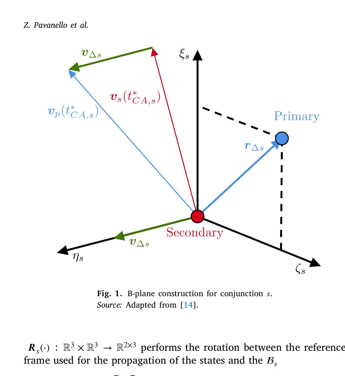
Figure 1: B-plane construction. Source: Adapted from [Armellin, 2021]
Under the short-term encounter hypothesis, relative motion can be approximated as uniform rectilinear. The Probability of Collision (PoC) computation reduces to a 2D integral over the combined covariance ellipse in the B-plane:
$$ P_{C,s} = \frac{1}{\sqrt{(2\pi)^3 \det(\boldsymbol{P}_{\mathcal{B}_s})}} \iint_{C_{HBR}} e^{-d_{m,s}^2/2} \, dA $$
where $d_{m,s}^2 = \boldsymbol{r}_{\mathcal{B}_s}^T \boldsymbol{P}_{\mathcal{B}_s}^{-1} \boldsymbol{r}_{\mathcal{B}_s}$ is the squared Mahalanobis distance of the relative position in the B-plane, and $C_{HBR}$ is the combined hard-body radius circle.
The paper uses Chan's method to approximate this integral, but explicitly notes that the optimisation method is independent of the specific PoC model — DA can automatically handle any functional form.
2.3 Multiple Operational Constraints
A distinctive feature of the paper is the unified treatment of diverse operational constraints:
(1) Collision Avoidance Constraints:
- Single-conjunction PoC: $P_{C,s} \leq \bar{P}_C$
- Total PoC (TPoC) for multiple conjunctions: $P_C = 1 - \prod_{s=1}^{n_{conj}} (1 - P_{C,s})$
- Miss Distance (MD): $d_{miss,s}^2 = \|\boldsymbol{r}_{\mathcal{B}_s}\|^2 \geq \bar{d}^2$
(2) Station-Keeping (SK) Constraints:
Two alternative formulations:
- Osculating Keplerian elements: require post-manoeuvre recovery of semi-major axis, eccentricity, inclination, argument of perigee, and RAAN to nominal values
- Mean orbital elements: constrain only mean semi-major axis and eccentricity deviations within thresholds, more practical for operations
$$ \varepsilon_{sma} = (a_m(t_f) - \bar{a}_m(t_f))^2 \leq \Delta a_{max}^2 $$
$$ \varepsilon_{ecc} = (e_m(t_f) - \bar{e}_m(t_f))^2 \leq \Delta e_{max}^2 $$
3. Core Method: From Polynomial Programming to Recursive Linearisation
3.1 Differential Algebra (DA) and Polynomial Programming (PP)
Differential Algebra is the technical foundation of this method. In essence, DA automatically tracks and propagates high-order derivative information during numerical computations. While a conventional orbit propagator outputs only numerical state values, a DA-enhanced propagator outputs Taylor polynomial expansions of the state with respect to the control variables.
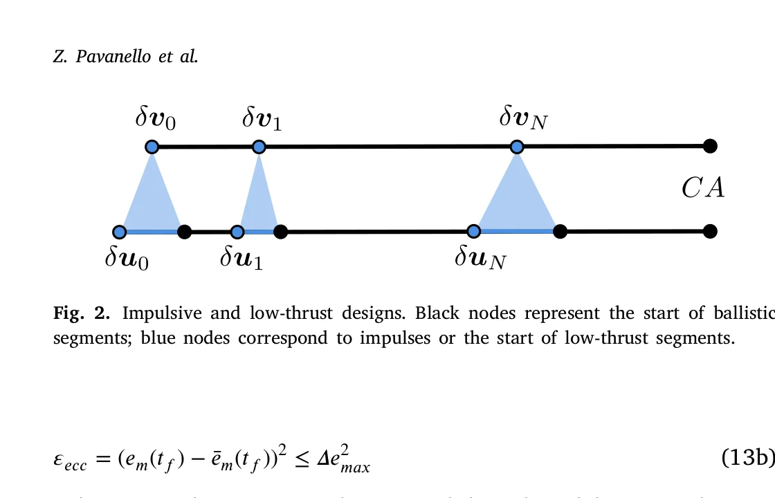
Figure 2: Impulsive and low-thrust designs. Black nodes represent the start of ballistic segments; blue nodes correspond to impulses or the start of low-thrust segments.
Through DA forward propagation, any state-dependent scalar constraint function $h(\boldsymbol{\Phi})$ (e.g., PoC, MD, orbital element deviation) can be expanded as an $n$-th order polynomial in the control variables $\boldsymbol{\Phi}$:
$$ \mathcal{T}_h^n(\boldsymbol{\Phi}) = h_0 + \sum_{k=1}^{n} \mathcal{H}^{(k)} \boldsymbol{\Phi}^k $$
where $\mathcal{H}^{(k)}$ is a $k$-th order supersymmetric tensor encoding the $k$-th order partial derivatives of $h$ with respect to $\boldsymbol{\Phi}$.
The CAM optimisation problem is thus transcribed as the following Polynomial Programme (PP):
$$ \begin{aligned} \min_{\boldsymbol{\Phi}} \quad & \boldsymbol{\Phi}^T \boldsymbol{\Phi} \\ \text{s.t.} \quad & \sum_{k=1}^{n} \mathcal{G}_v^{(k)} \boldsymbol{\Phi}^k \leq \rho_v, \quad v \in \{1, \ldots, n_{in}\} \\ & \sum_{k=1}^{n} \mathcal{H}_c^{(k)} \boldsymbol{\Phi}^k = \rho_c, \quad c \in \{1, \ldots, n_{eq}\} \end{aligned} $$
The objective is $\boldsymbol{\Phi}^T\boldsymbol{\Phi}$ (energy-optimal), and the constraints are $n$-th order polynomial inequalities and equalities.
3.2 The Recursive Polynomial Method
Directly solving the high-order PP is extremely difficult. The paper's key innovation is to convert it into an iterative sequence of Quadratic Programs (QPs).
Step 1 — First-order truncation: Truncate all polynomial constraints to first order, yielding a QP:
$$ \begin{aligned} \min_{\boldsymbol{\Phi}} \quad & \boldsymbol{\Phi}^T \boldsymbol{\Phi} \\ \text{s.t.} \quad & \mathcal{H}_v^{(1)} \boldsymbol{\Phi} \leq \rho_v, \quad \mathcal{H}_c^{(1)} \boldsymbol{\Phi} = \rho_c \end{aligned} $$
Using interior-point or active-set methods, the optimal QP solution $[\boldsymbol{\Phi}]_1$ can be found in polynomial time.
Step 2 — Higher-order recursion: Given the $(j-1)$-th order optimal solution $[\boldsymbol{\Phi}]_{j-1}$, the higher-order terms of the $j$-th order PP are linearised at this point:
$$ \gamma_c^{(j)} := \mathcal{H}_c^{(1)} + \sum_{k=2}^{j} \mathcal{H}_c^{(k)} [\boldsymbol{\Phi}]_{j-1}^{k-1} $$
Here, $\gamma_c^{(j)}$ is termed the $j$-th order pseudo-gradient — it incorporates first-order corrections from higher-order terms evaluated at the current solution. The $j$-th order PP is thus approximated as a new QP:
$$ \min_{\boldsymbol{\Phi}} \quad \boldsymbol{\Phi}^T \boldsymbol{\Phi} \quad \text{s.t.} \quad \gamma_v^{(j)} \boldsymbol{\Phi} \leq \rho_v, \quad \gamma_c^{(j)} \boldsymbol{\Phi} = \rho_c $$
Solving this QP yields $[\boldsymbol{\Phi}]_j$, which then serves as the new linearisation point. The process repeats until convergence:
$$ \| [\boldsymbol{\Phi}]_j^b - [\boldsymbol{\Phi}]_j^{b-1} \|_2 \leq e_{tol} $$
After convergence at order $j$, the expansion order is incremented to $j+1$, and the entire process repeats up to order $n$.
Core advantages of the method:
-
Polynomial maps are computed only once. Unlike traditional Sequential Convex Programming (SCP), which requires re-propagation and re-linearisation at each iteration, the recursive method pre-computes all high-order polynomial coefficients in a single DA pass. All subsequent linearisation operations are purely algebraic.
-
Extremely low computational complexity. Each iteration only requires solving one QP (polynomial time), and overall convergence is fast (typically < 15 iterations).
-
Handles highly nonlinear constraints. When first-order truncation is insufficient, the recursive inclusion of higher-order terms systematically improves accuracy.
4. Experimental Validation: Comprehensive Multi-Scenario Assessment
The paper validates the method across multiple dimensions. All simulations were run on an Intel Core i7-11700 @2.5GHz using MATLAB R2024a and C++.
4.1 CAM + Osculating Keplerian Element Recovery (Section 6.1)
Using the ESA Collision Avoidance Challenge database of 2,170 real conjunction scenarios, with coupled PoC constraints and five-dimensional osculating Keplerian element recovery.
The manoeuvre scheme uses bi-impulsive control: the first impulse at 0.5 orbital periods before TCA, and the second at 0.5 orbital periods after TCA to recover the nominal orbit.
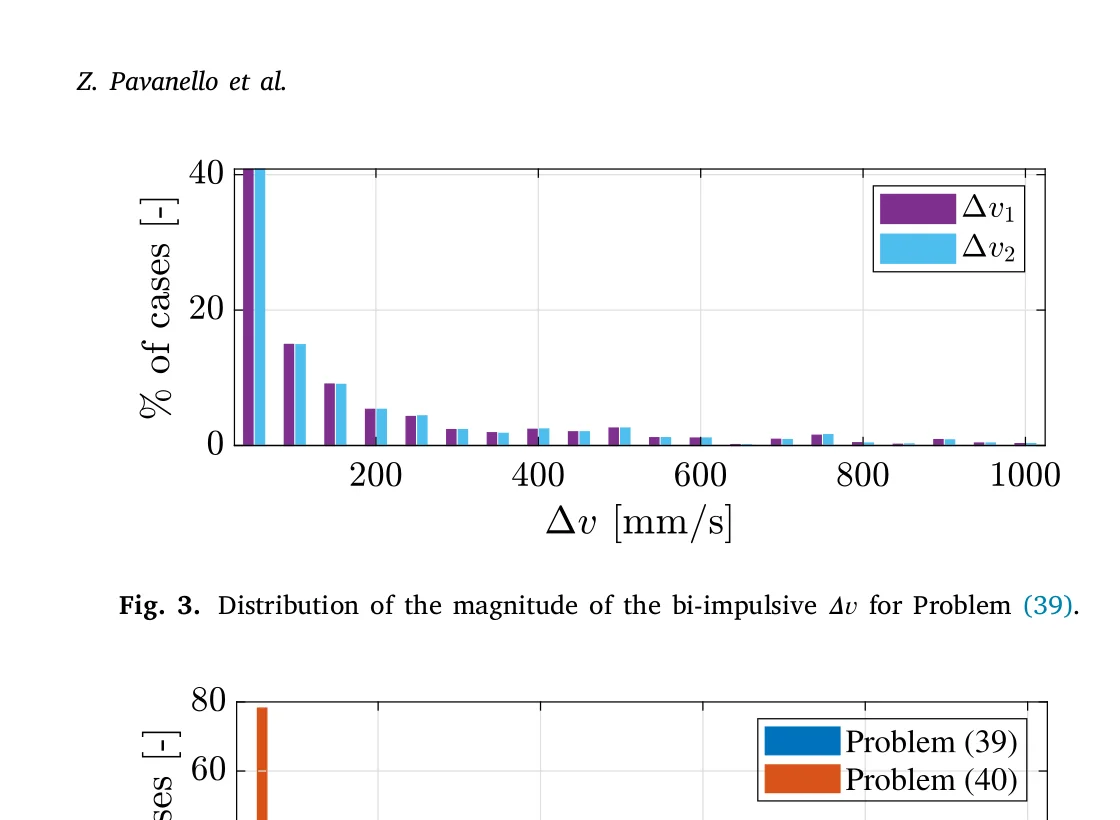
Figure 3: Distribution of bi-impulsive Δv magnitude (Problem 39). Most scenarios require < 50 mm/s; extreme cases up to ~1 m/s.
Key results:
- Total Δv: Vast majority of scenarios < 50 mm/s; extreme cases up to ~1 m/s
- PoC relative error: Maximum absolute error only $4 \times 10^{-9}$
- Orbit recovery error: Position < 2 cm, velocity < 0.15 mm/s
- Computation time: 95th percentile < 0.15 s
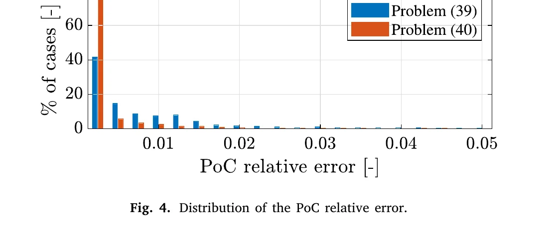
Figure 4: Distribution of the PoC relative error. Blue bars correspond to Problem (39) (osculating element recovery), orange bars to Problem (40) (mean element recovery). Problem (40) exhibits a much higher concentration near zero error, with nearly 80% of cases showing negligible PoC error.
Figure 4 reveals the difference in PoC constraint accuracy between the two SK strategies. Problem (40), with its more relaxed constraints (only mean semi-major axis and eccentricity), gives the optimiser a larger feasible region to find low-PoC solutions, resulting in an extremely high concentration near zero error. In contrast, Problem (39) with five-dimensional osculating element recovery shows a more dispersed PoC error distribution due to tighter constraints.
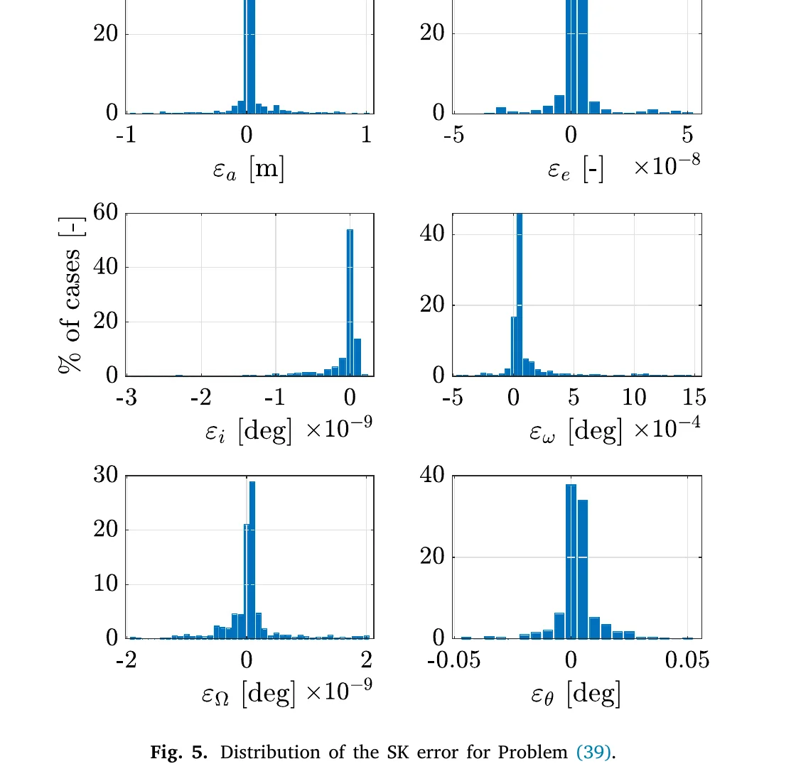
Figure 5: Distribution of the SK error for Problem (39). Six subplots show the error distributions for semi-major axis a, eccentricity e, inclination i, argument of perigee ω, RAAN Ω, and true anomaly θ. All errors are tightly concentrated around zero, validating the high-precision satisfaction of SK constraints.
Figure 5 provides a comprehensive view of the five-dimensional osculating Keplerian element recovery accuracy. Notably, the error distributions for all elements are extremely narrow — semi-major axis errors within ±1 m and angular errors on the order of 10⁻⁴ degrees — fully demonstrating the recursive method's ability to strictly satisfy osculating-element SK constraints.
4.2 CAM + Mean Orbital Element Recovery (Section 6.2)
Relaxing SK constraints to only control mean semi-major axis error ≤ 3 m and eccentricity error ≤ 3 m. With less stringent requirements, total Δv is significantly reduced.
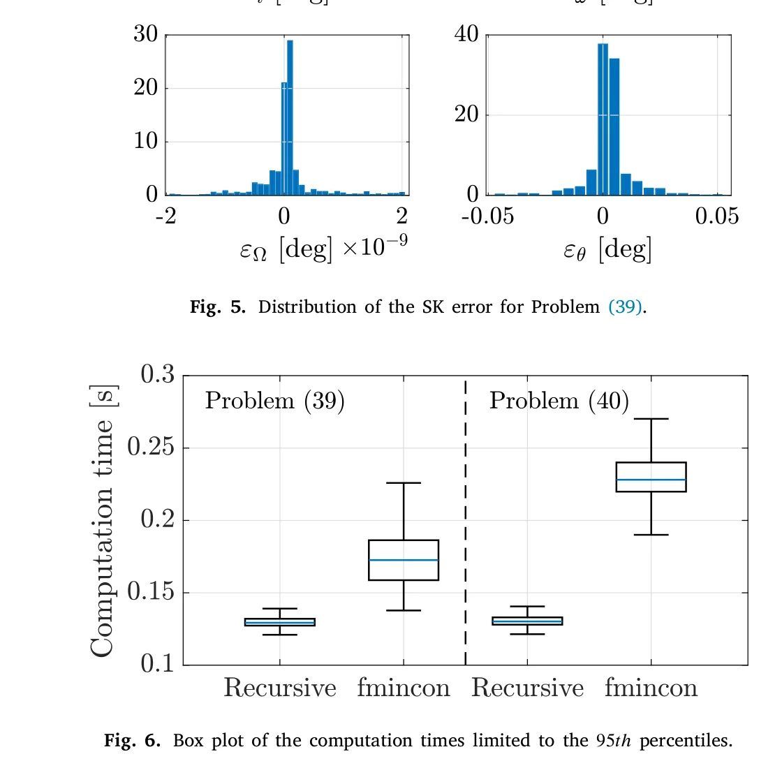
Figure 6: Box plot of computation times limited to the 95th percentiles. The recursive method significantly outperforms MATLAB fmincon.
Comparison with fmincon:
- Problem (39) (osculating elements): Recursive method 30% faster on average
- Problem (40) (mean elements): Recursive method 40% faster on average
- Recursive method exhibits significantly tighter time distribution and greater reliability
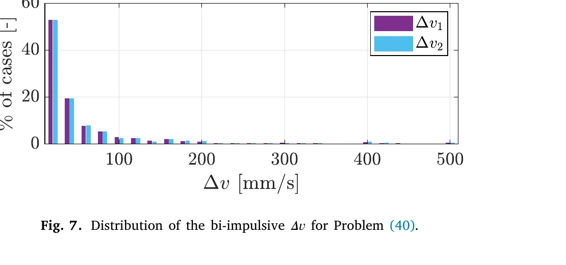
Figure 7: Distribution of the bi-impulsive Δv magnitude for Problem (40). Purple bars = Δv₁ (pre-conjunction impulse), light blue bars = Δv₂ (post-conjunction impulse). The vast majority of cases require well under 100 mm/s, substantially lower than Problem (39).
Comparing Figure 7 with Figure 3 clearly shows that relaxing the SK constraints significantly reduces total Δv. Problem (40) only requires recovery of mean semi-major axis (≤ 3 m) and eccentricity (≤ 3 m), without mandating recovery of inclination, argument of perigee, or RAAN, allowing the optimiser to employ more fuel-efficient tangential impulses.
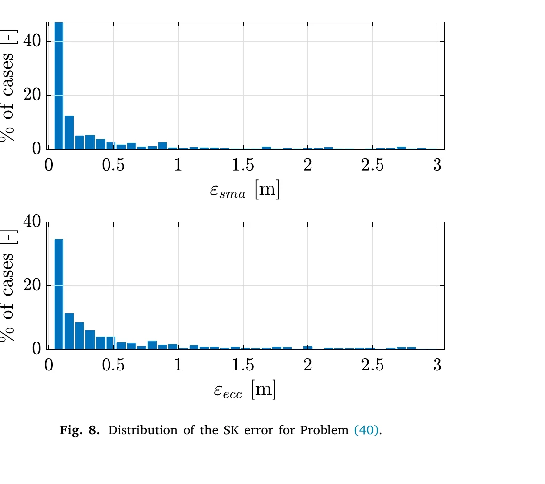
Figure 8: Distribution of the SK error for Problem (40). Top: mean semi-major axis error ε_sma; bottom: eccentricity error ε_ecc. Both are strictly bounded within 3 m, with the vast majority of cases showing near-zero error.
Figure 8 validates the satisfaction of mean-element SK constraints. Both histograms exhibit highly right-skewed distributions — the overwhelming majority of cases recover semi-major axis and eccentricity with near-zero error, with only a tiny fraction approaching the 3 m tolerance bound. This demonstrates that the recursive method maintains strong constraint satisfaction even under relaxed requirements.
4.3 Multiple Encounters (Section 6.3)
A primary LEO satellite facing 2–3 consecutive encounters with different secondaries. The paper compares three different collision metrics: TPoC, individual PoC, and MD.
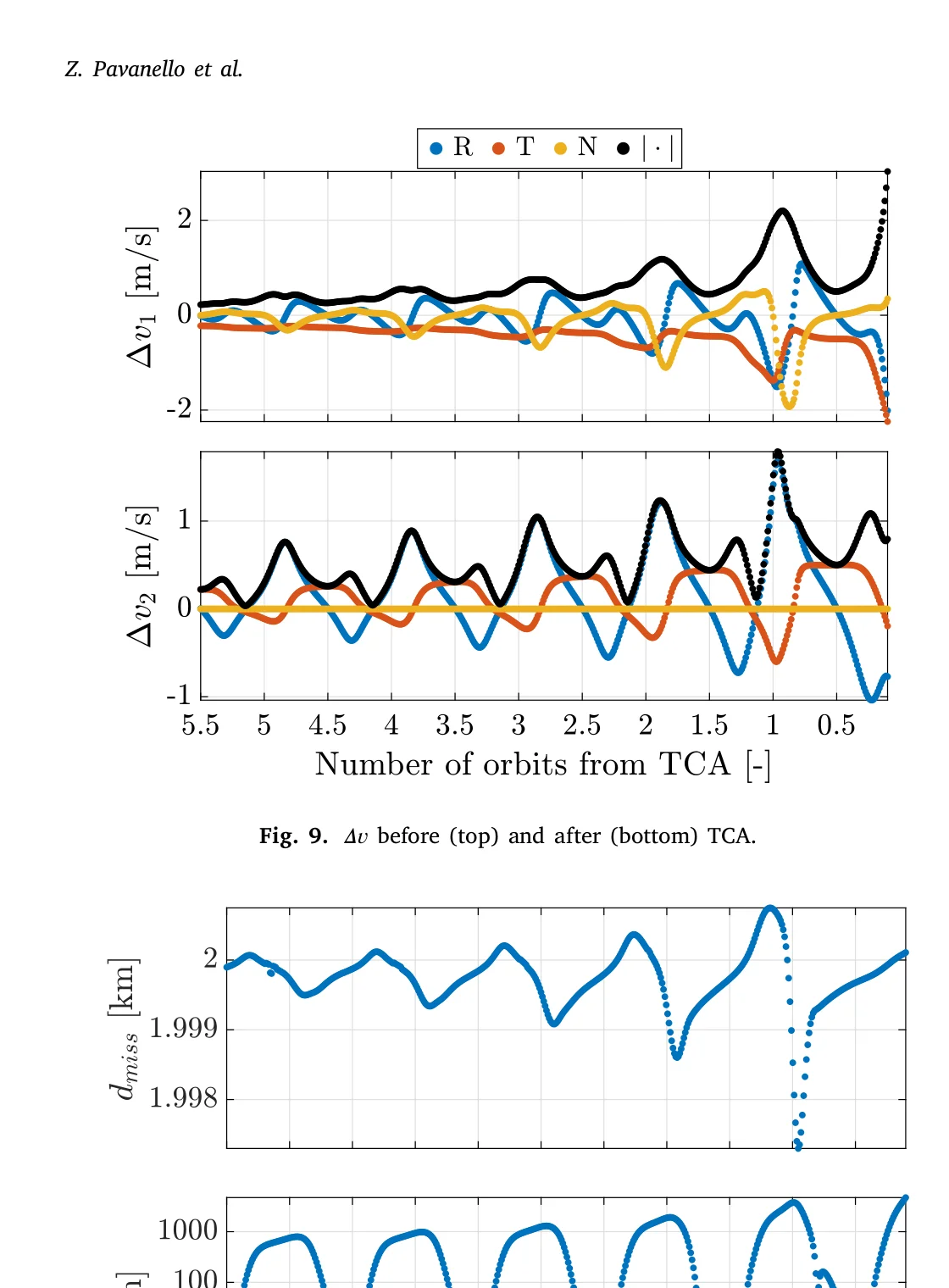
Figure 9: Δv before (top) and after (bottom) TCA. Firing at half-orbit intervals yields optimal fuel efficiency.
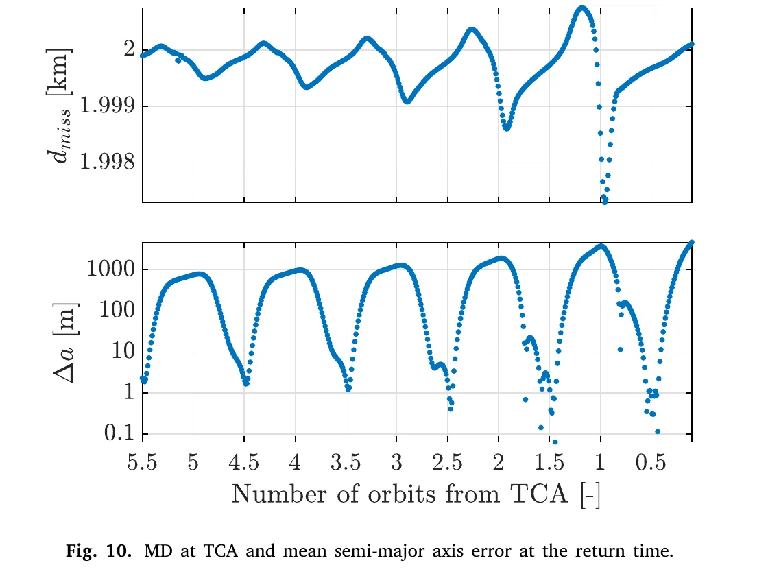
Figure 10: Miss distance at TCA (top) and mean semi-major axis error at the return time (bottom) as functions of the firing orbit count. The top plot shows d_miss oscillating around the 2 km threshold; the bottom plot uses a logarithmic scale to show Δa dropping to acceptable levels (< 10 m) only when firing at integer multiples of half orbital periods.
Figure 10 provides visual evidence from the parametric sweep analysis for the multi-encounter scenario. The top plot confirms that d_miss can be precisely maintained near the 2 km MD threshold when firing at optimal times (integer multiples of half orbital periods). The bottom plot, using a logarithmic scale, dramatically illustrates the semi-major axis error's sensitivity to firing timing — only at optimal timings (5.5, 4.5, 3.5, ..., 0.5 orbits before conjunction) does Δa fall within reasonable bounds (< 10 m).
Key findings:
- Optimal firing times: Multiples of 0.5 orbital periods before conjunction
- Worst firing times: Around 3/4 of the orbital period (require large out-of-plane components)
- TPoC and individual PoC constraints produce nearly identical optimal manoeuvres
- MD constraint yields higher Δv because the manoeuvre must achieve a larger separation
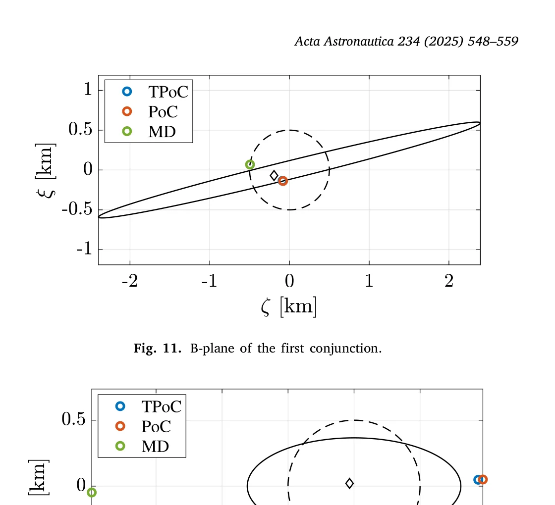
Figure 11: B-plane of the first conjunction. Solid ellipse: iso-probability ellipse for PoC = 10⁻⁶; dashed circle: MD threshold.
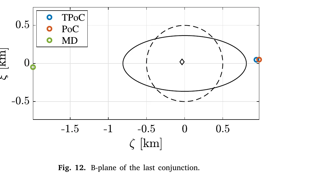
Figure 12: B-plane of the last conjunction. In contrast with Figure 11: for the last conjunction, the PoC (orange) and TPoC (blue) optimal solutions lie at the far-right edge of the iso-probability ellipse, while the MD (green) solution is located far to the left, away from the main ellipse body.
The contrast between Figures 11 and 12 reveals the core challenge of multi-conjunction scenarios. In the first conjunction, the optimal solutions for all three metrics (TPoC, PoC, MD) are relatively close in the B-plane. However, for the last conjunction, the MD-optimal solution points in the opposite direction from the PoC/TPoC solutions — meaning a manoeuvre that avoids one conjunction may be detrimental to another, underscoring the necessity of global optimisation.
4.4 Multiple Encounters + SK + Low-Thrust (Section 6.4)
The most challenging scenario: three consecutive conjunctions + mean orbital element recovery + low-thrust dynamics. Three continuous thrust arcs are employed; expansion order is 4.
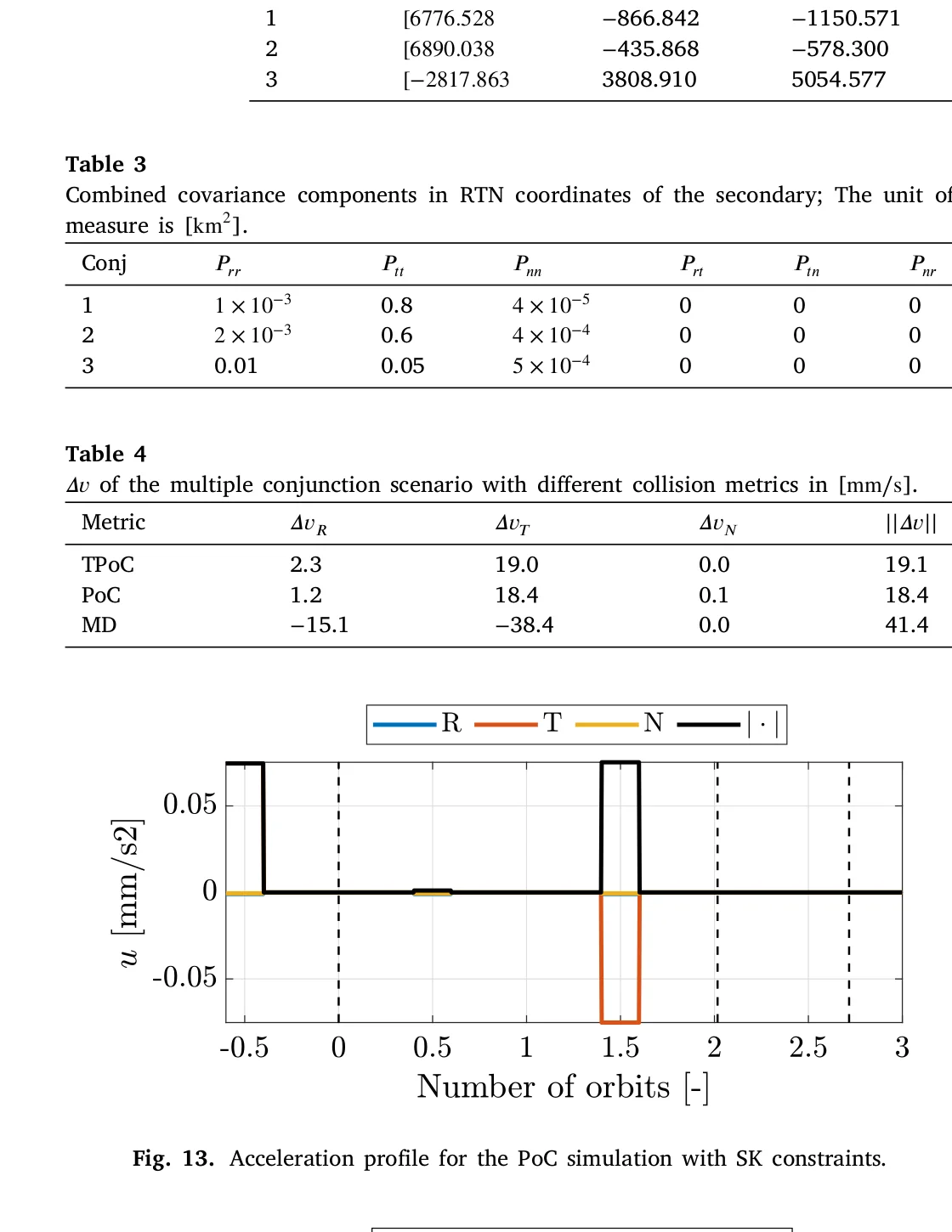
Figures 13 & 14: Low-thrust acceleration profiles for PoC (left) and MD (right) optimisation with SK constraints.
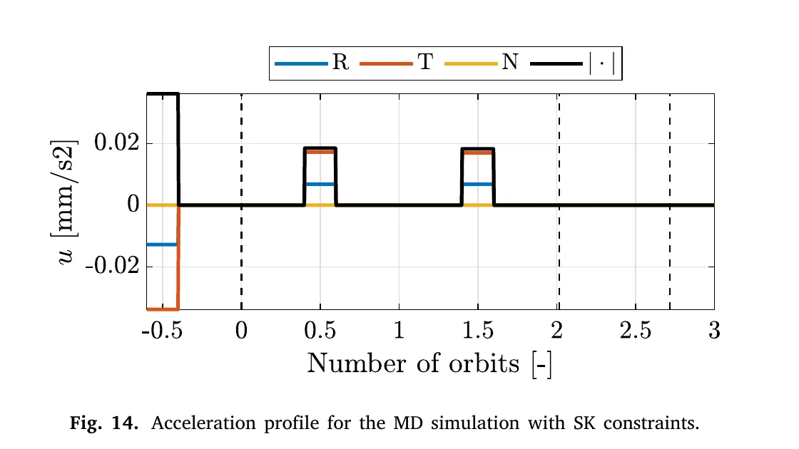
Figure 14: Low-thrust acceleration profile for the MD optimisation with SK constraints. Blue/orange/yellow lines represent radial (R), transverse (T), and normal (N) components respectively; the black line is total magnitude. Pulses are concentrated around orbits -0.5, 0.5, and 1.5.
Comparing Figures 13 and 14 reveals the distinct low-thrust profiles corresponding to PoC and MD collision metrics. The PoC optimisation requires higher acceleration peaks (~0.05 mm/s²), while MD optimisation peaks are lower (~0.03 mm/s²). Both share similar thrust window positions (at -0.5, 0.5, 1.5 orbital periods), but differ in directional allocation — reflecting how different collision metrics guide trajectories differently in the B-plane.
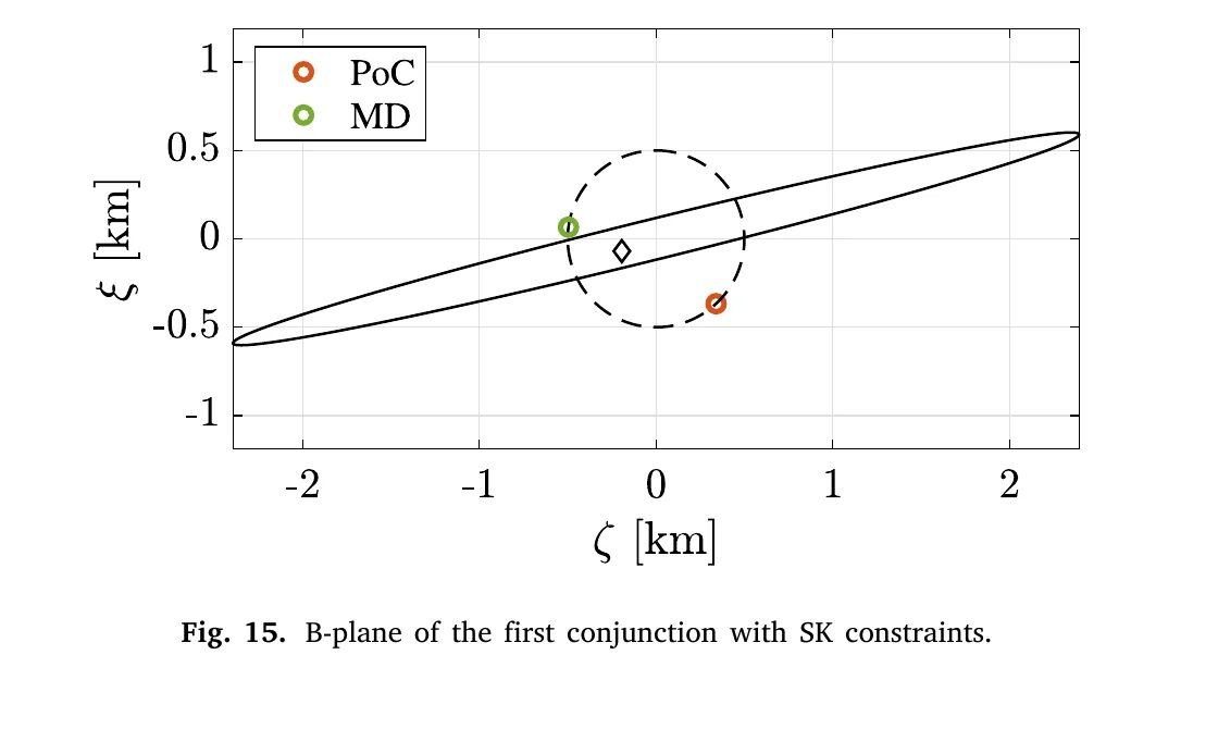
Figure 15: B-plane of the first conjunction with SK constraints. Orange (PoC) and green (MD) markers show the B-plane mapping points under the two strategies. Black curves represent the relative motion trajectory; the dashed circle is the combined hard-body radius.
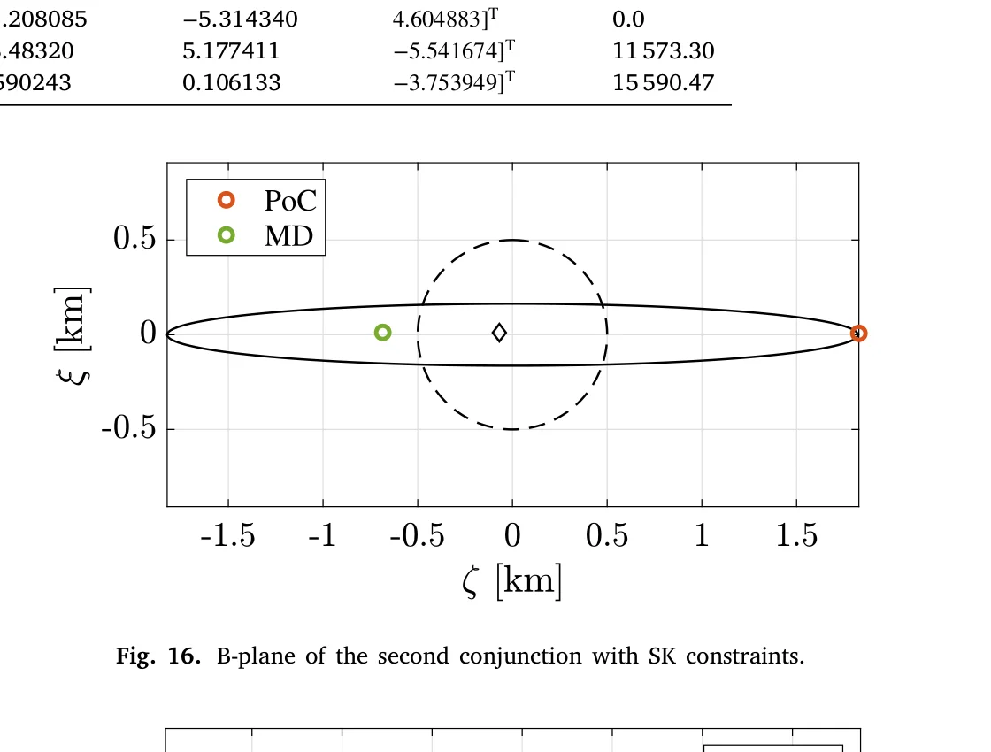
Figure 16: B-plane of the second conjunction with SK constraints. Note the highly elongated iso-probability ellipse.
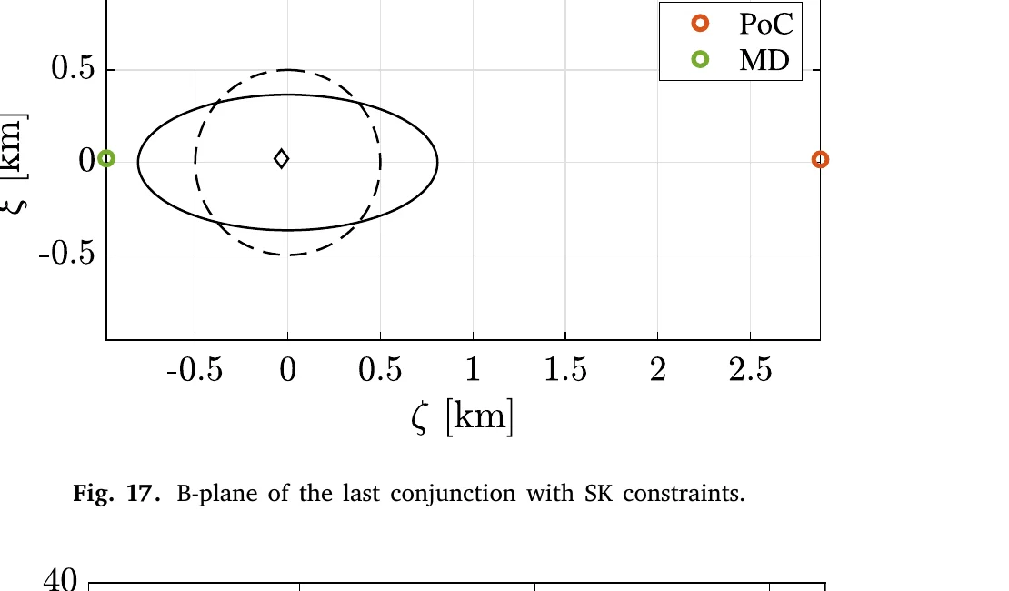
Figure 17: B-plane of the last conjunction with SK constraints. In contrast with Figure 16, this conjunction's constraint is inactive — both PoC and MD optimal solutions lie well inside the iso-probability ellipse, indicating that this encounter does not impose an active constraint on the optimisation.
Figure 17 reveals an important phenomenon: in three-conjunction scenarios, not all conjunction constraints are active. The last conjunction's iso-probability ellipse completely encloses the dashed safety circle, and both PoC and MD optimal solutions lie safely within the ellipse — meaning the optimiser does not need to allocate control resources specifically for this encounter, as safety is naturally satisfied. This insight is significant for understanding the activation/dormancy mechanisms of constraints in multi-conjunction scenarios.
Core insights:
- In multi-conjunction scenarios, the optimal manoeuvre is not trivially a pure tangential burn — global optimisation is essential
- The constraint of the second conjunction is active; the optimal solution lies on the semi-major axis of the ellipse (direction of minimum PoC gradient)
- SK constraint accuracy reaches 11 mm for semi-major axis and 3.9 m for eccentricity
4.5 Convergence Analysis (Section 6.5)
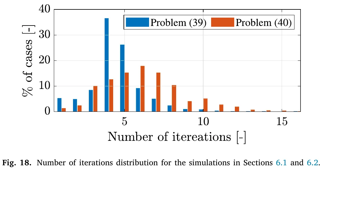
Figure 18: Distribution of the number of iterations for Problems (39) and (40). The recursive method converges in fewer than 15 iterations for all single-conjunction scenarios, demonstrating robust and predictable convergence behaviour.
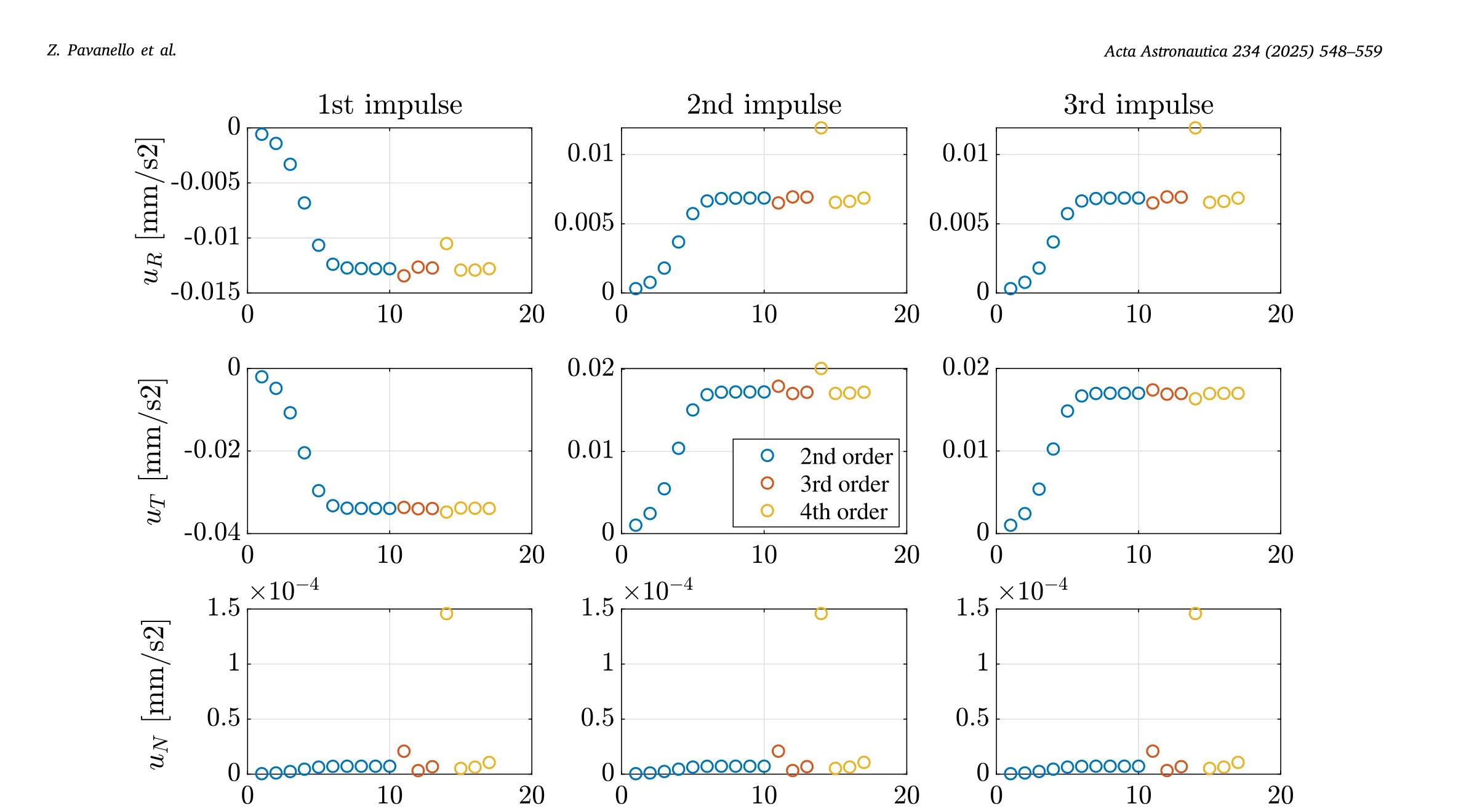
Figure 19: Evolution of each control acceleration component across iterations. Blue/orange/yellow dots correspond to 2nd/3rd/4th order expansions.
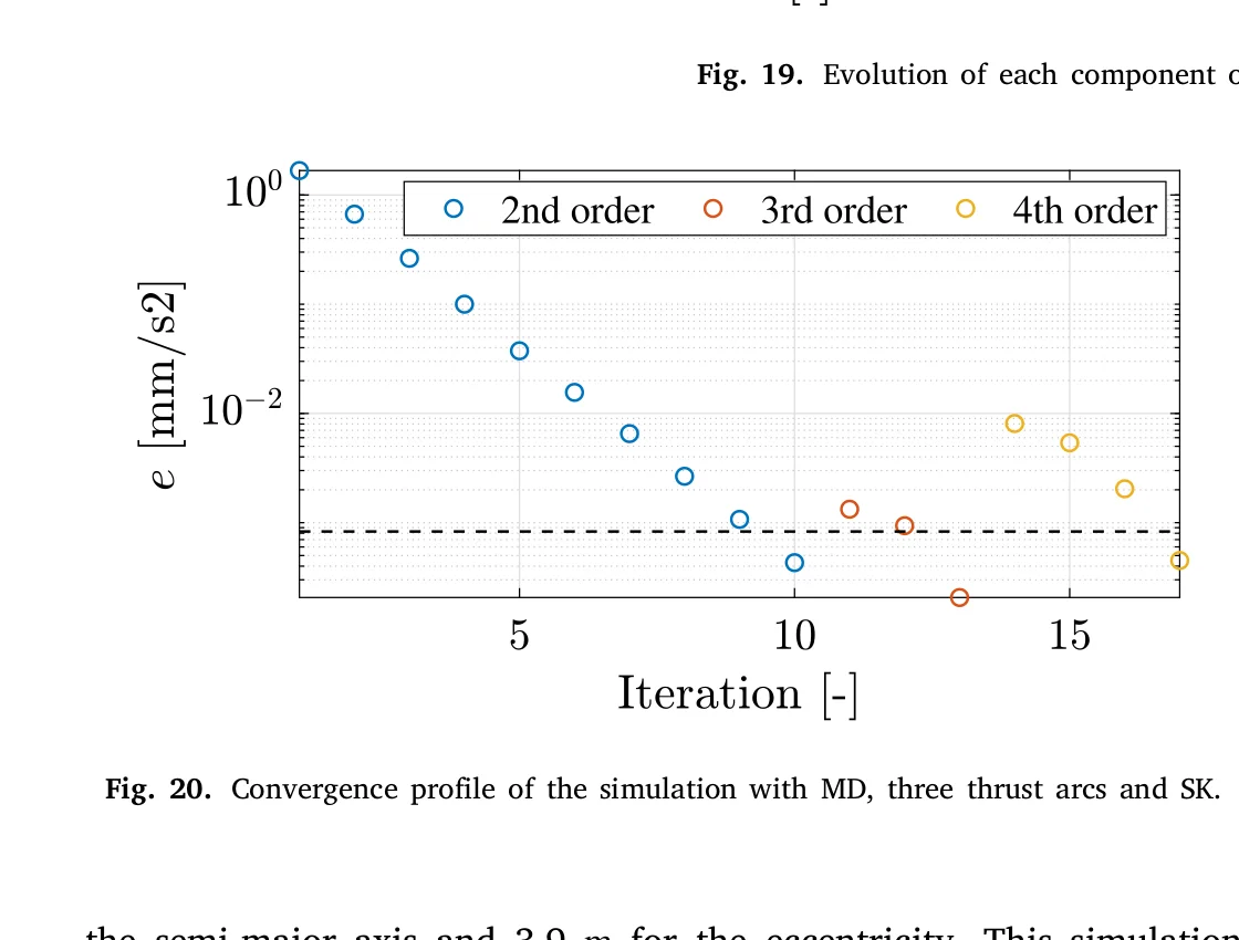
Figure 20: Convergence profile for the simulation with MD, three thrust arcs, and SK.
Convergence characteristics:
- Problem (39)/(40) (single conjunction + SK): Always < 15 iterations
- Multi-conjunction + low-thrust scenarios: 14–33 iterations required
- Most iterations are spent transitioning from first-order to second-order solutions (convergence around the 11th iteration)
- Third- and fourth-order expansions yield solutions very similar to second-order — a second-order expansion is often sufficient in practice
5. Method Comparison and Discussion
5.1 Comparison with fmincon
| Metric | Recursive Method | fmincon (Interior-Point) |
|---|---|---|
| Avg. computation time (Problem 39) | Baseline | 30% slower |
| Avg. computation time (Problem 40) | Baseline | 40% slower |
| Time distribution consistency | ✅ Tight | ❌ Dispersed |
| Convergence reliability | ✅ Stable | ⚠️ Occasional fluctuation |
| Gradient computation | Automatic (DA) | Numerical differencing |
5.2 Comparison with Sequential Convex Programming (SCP)
Traditional SCP requires re-building linear maps from a new expansion point at each iteration (re-propagation + re-linearisation). In contrast, the recursive method computes the polynomial maps only once during the initial DA pass — all subsequent linearisation operations are purely algebraic, dramatically reducing computational load.
5.3 Scope of Applicability
The paper emphasises the method's generality:
- ✅ Single / multiple conjunctions
- ✅ PoC / MD / TPoC collision metrics
- ✅ Impulsive / multi-impulsive / low-thrust dynamics
- ✅ Osculating / mean orbital element SK constraints
- ✅ Compatible with any PoC computation model
- ✅ Compatible with any dynamical model
6. Conclusions and Engineering Significance
This paper presents a simple, efficient, and general method for CAM optimisation:
- Differential Algebra automatically constructs high-order Taylor polynomials of constraints (PoC, MD, SK) with respect to the control
- CAM is formulated as an energy-optimal Polynomial Programme (PP)
- Recursive linearisation converts the high-order PP into an iterative sequence of Quadratic Programs (QPs)
- Polynomial maps are computed only once — subsequent iterations are purely algebraic, maximising efficiency
Numerical results are impressive:
- Extremely fast: CAM+SK optimisation for 2,170 real conjunction scenarios completes within 0.1–0.5 seconds
- Highly accurate: PoC constraint error as low as $4 \times 10^{-9}$; orbit recovery error < 2 cm
- Outperforms general-purpose solvers: Recursive method 30–40% faster on average than MATLAB fmincon, with tighter time distributions
- Highly general: Simultaneously supports impulsive/low-thrust dynamics, PoC/MD metrics, and multiple SK constraint types
Engineering Prospects
From an engineering perspective, this work carries significance on multiple levels:
-
Autonomous space traffic management. The 0.1–0.5 s computation time enables potential onboard autonomous computation, dramatically reducing dependence on ground operators.
-
Multi-conjunction scenarios. As orbits become increasingly congested, single satellites simultaneously facing multiple conjunction warnings is becoming the norm. This method can design optimal avoidance strategies for multi-conjunction scenarios within a unified framework.
-
Integrated manoeuvre-and-recovery. Coupling CAM with orbit recovery into a single optimisation problem avoids the suboptimal "avoid first, recover later" strategy.
-
Broad compatibility. Through DA's automation, the method is decoupled from specific PoC and dynamical models — adapting to different mission requirements only requires swapping the propagator.
Limitations
Notable limitations include:
- Impulse/thrust timing must be pre-specified (the paper validates half-orbital-period multiples as optimal via parametric sweep)
- High-order expansion accuracy may degrade under extreme nonlinearity
- Currently validated only for LEO short-term encounter scenarios
References
- Z. Pavanello, L. Pirovano, R. Armellin, "Efficient collision avoidance manoeuvres under multiple polynomial constraints," Acta Astronautica, vol. 234, pp. 548–559, 2025. DOI: 10.1016/j.actaastro.2025.05.002
- R. Armellin, "Collision avoidance maneuver optimization with a multiple-impulse convex formulation," Acta Astronautica, vol. 186, pp. 347–362, 2021.
- C. Bombardelli, J. Hernando-Ayuso, "Optimal impulsive collision avoidance in low earth orbit," Journal of Guidance, Control, and Dynamics, vol. 38, no. 2, pp. 217–225, 2015.
- Z. Pavanello, L. Pirovano, R. Armellin, "Recursive Polynomial Method for Fast Collision Avoidance Maneuver Design," IEEE Transactions on Aerospace and Electronic Systems, vol. 61, no. 2, pp. 2914–2925, 2025.
- S. Dutta, A.K. Misra, "Convex optimization of collision avoidance maneuvers in the presence of uncertainty," Acta Astronautica, vol. 197, pp. 257–268, 2022.
This is the inaugural article of the "Cutting-Edge Tech Exploration" column. This column focuses on tracking and interpreting recently published (2023–2026) cutting-edge technical papers, emphasising methodological innovation and engineering application value, aiming to provide readers with timely academic frontier updates and in-depth technical analysis.