[Classic Paper Review] Proximal Policy Optimization — From TRPO to PPO Clip
2026-07-01
Proximal Policy Optimization — From TRPO to PPO Clip
Paper: John Schulman, Filip Wolski, Prafulla Dhariwal, Alec Radford, Oleg Klimov. "Proximal Policy Optimization Algorithms." arXiv preprint arXiv:1707.06347v2, 2017.
Affiliation: OpenAI
1. Introduction: The "Trilemma" of RL Algorithms
Before 2017, reinforcement learning methods using neural network function approximators fell broadly into three "schools":
- DQN (Deep Q-Learning): Sample-efficient, but struggles with continuous action spaces (e.g., robot control) and lacks theoretical guarantees;
- VPG (Vanilla Policy Gradient): Simple to implement and widely applicable, but suffers from poor sample efficiency and hyperparameter sensitivity — a single gradient update can catastrophically "break" the policy;
- TRPO (Trust Region Policy Optimization): Guarantees monotonic policy improvement through trust-region constraints, but is complex to implement — requiring conjugate gradient algorithms, quadratic approximations, and line search — and is incompatible with architectures involving dropout or policy-value network parameter sharing.
Each approach has its strengths, but none simultaneously satisfies all three desiderata:
- 🔧 Easy to implement (scalable to large models and parallel implementations)
- 📊 Data efficient
- 🎯 Robust (without extensive hyperparameter tuning)
This is precisely the motivation behind Schulman et al.'s Proximal Policy Optimization (PPO) : can we design an algorithm that combines TRPO's data efficiency and stability with the simplicity of first-order optimization (like VPG), while also being compatible with more general network architectures?
The answer is: PPO Clip — through a cleverly designed clipped surrogate objective, requiring only a few lines of code change to a standard policy gradient implementation, PPO achieves all three goals.
2. Background: Policy Gradients and the TRPO Dilemma
2.1 The Limitations of Vanilla Policy Gradient
The core idea of policy gradient methods is intuitive: directly differentiate the policy $\pi_\theta$ with respect to its parameters $\theta$ to maximize expected returns. The most commonly used gradient estimator is:
$$\hat{g} = \hat{\mathbb{E}}_t \left[ \nabla_\theta \log \pi_\theta(a_t | s_t) \hat{A}_t \right] \tag{1}$$
where $\hat{A}_t$ is an estimator of the advantage function. The corresponding objective function is:
$$L^{PG}(\theta) = \hat{\mathbb{E}}_t \left[ \log \pi_\theta(a_t | s_t) \hat{A}_t \right] \tag{2}$$
Intuitively: if an action has positive advantage ("better than average"), we increase its probability; if negative, we decrease it.
Here's the catch: performing multiple steps of optimization on $L^{PG}$ using the same batch of data has no theoretical justification. In practice, doing so often leads to destructively large policy updates — the policy parameters drift far from the "valid region," causing performance to collapse. Consequently, standard VPG can only perform one gradient update per batch of data, resulting in extremely poor sample efficiency.
2.2 TRPO: The Cost of Trust-Region Constraints
TRPO addresses this problem by maximizing the objective function while imposing a hard constraint on the "magnitude" of the policy update. Specifically:
$$\underset{\theta}{\text{maximize}} \ \hat{\mathbb{E}}_t \left[ \frac{\pi_\theta(a_t | s_t)}{\pi_{\theta_{old}}(a_t | s_t)} \hat{A}_t \right] \tag{3}$$
$$\text{subject to} \ \hat{\mathbb{E}}_t \left[ \text{KL}[\pi_{\theta_{old}}(\cdot | s_t), \pi_\theta(\cdot | s_t)] \right] \leq \delta \tag{4}$$
where $\theta_{old}$ denotes the policy parameters before the update, and $\delta$ is the KL divergence constraint threshold. This constraint ensures the new policy does not stray too far from the old one, providing a theoretical guarantee of monotonic improvement.
But at what cost?
- 🧮 Implementation complexity: TRPO requires a linear approximation of the objective, a quadratic approximation of the constraint, and solving the resulting problem via conjugate gradient;
- 🚫 Architectural limitations: Dropout is incompatible (noise destabilizes KL estimates), and parameter sharing between policy and value networks is unsupported;
- 🔬 Debugging burden: Additional hyperparameters such as line search parameters and damping coefficients increase engineering overhead.
💡 Key Insight: TRPO's underlying theory actually suggests using a KL penalty rather than a hard constraint:
$$\underset{\theta}{\text{maximize}} \ \hat{\mathbb{E}}_t \left[ \frac{\pi_\theta(a_t | s_t)}{\pi_{\theta_{old}}(a_t | s_t)} \hat{A}_t - \beta \ \text{KL}[\pi_{\theta_{old}}(\cdot | s_t), \pi_\theta(\cdot | s_t)] \right] \tag{5}$$
The problem: a single value of $\beta$ fails to perform well across different problems — or even within a single problem as its characteristics evolve during training. This is why TRPO resorts to a hard constraint. PPO's central contribution is finding a more elegant alternative.
3. Clipped Surrogate Objective: The Core Innovation of PPO 🎯
3.1 Probability Ratio and the CPI Objective
Define the probability ratio:
$$r_t(\theta) = \frac{\pi_\theta(a_t | s_t)}{\pi_{\theta_{old}}(a_t | s_t)}$$
Clearly $r(\theta_{old}) = 1$. TRPO maximizes the "surrogate" objective:
$$L^{CPI}(\theta) = \hat{\mathbb{E}}_t \left[ r_t(\theta) \hat{A}_t \right] \tag{6}$$
CPI stands for Conservative Policy Iteration [KL02]. $L^{CPI}$ is essentially the policy gradient objective reweighted by importance sampling. Maximizing it without constraints would cause $r_t(\theta)$ to explode far beyond 1, collapsing the policy.
3.2 The Motivation and Mathematical Form of Clipping
PPO's core innovation is the clipped surrogate objective:
$$L^{CLIP}(\theta) = \hat{\mathbb{E}}_t \left[ \min\left( r_t(\theta) \hat{A}_t, \ \text{clip}(r_t(\theta), 1 - \epsilon, 1 + \epsilon) \hat{A}_t \right) \right] \tag{7}$$
where $\epsilon$ is a hyperparameter (the paper recommends $\epsilon = 0.2$).
Let us unpack the intuition behind this formula layer by layer:
- First term $r_t(\theta) \hat{A}_t$: the standard CPI objective;
- Second term $\text{clip}(r_t(\theta), 1 - \epsilon, 1 + \epsilon) \hat{A}_t$: the surrogate objective with the probability ratio clipped to the interval $[1-\epsilon, 1+\epsilon]$;
- $\min(\cdot, \cdot)$: take the minimum of the two, making the final objective a pessimistic lower bound on the original objective.
👉 The key elegance of this design: clipping only takes effect when it would make the objective "improve"; when the objective would "worsen," clipping does not interfere.
Consider the two cases (see Figure 1):
| Case | Direction of $r_t$ change | Objective behavior | Effect |
|---|---|---|---|
| $A > 0$ (good action) | Want to increase $r_t$ | Clipped when $r_t > 1 + \epsilon$; objective stops growing | Prevents overconfidence in "good actions" |
| $A < 0$ (bad action) | Want to decrease $r_t$ | Clipped when $r_t < 1 - \epsilon$; objective stops decreasing | Prevents over-penalizing "bad actions" |
When $A > 0$, the $\min$ picks the clipped term (because it is lower), preventing $r_t$ from growing without bound. When $A < 0$, the $\min$ also picks the clipped term (because it is less "negative"), preventing $r_t$ from shrinking without bound.
💡 Core Intuition: PPO does not prevent you from adjusting probabilities in the "right direction" — it merely prevents you from adjusting too much at once. Think of it as a good coach: encouraging progress, but never letting you injure yourself by overdoing it in a single session.
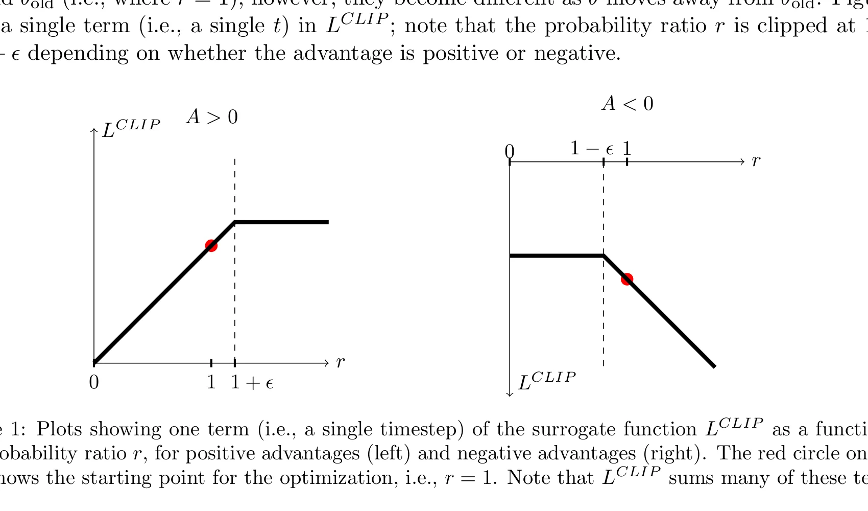
Figure 1 illustrates a single term of $L^{CLIP}$ as a function of the probability ratio $r$, for positive advantages (left) and negative advantages (right). The red dot marks the starting point $r=1$ (the policy before the update). Observe that $L^{CLIP}$ coincides with $L^{CPI}$ within the interval $[1-\epsilon, 1+\epsilon]$ but is "flattened" outside it.
4. Visualizing the Mechanism of PPO 📊
4.1 Interpolating Surrogate Objectives Along the Update Direction
Figure 2 provides another important perspective for understanding $L^{CLIP}$'s behavior. It shows how various objectives vary as we interpolate along the policy update direction during one iteration of PPO:
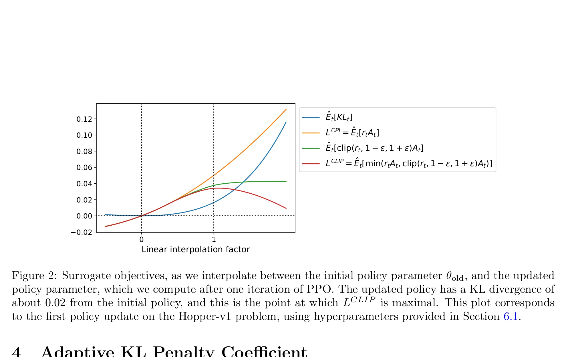
Figure 2 is from the first policy update on the Hopper-v1 task:
- Blue curve ($\hat{\mathbb{E}}_t[KL_t]$): KL divergence grows rapidly as the interpolation factor increases;
- Orange curve ($L^{CPI}$): the unconstrained objective grows linearly without bound — this would lead to excessively large policy updates;
- Green curve ($\hat{\mathbb{E}}_t[\text{clip}]$): the clipped term flattens once the policy deviates sufficiently;
- Red curve ($L^{CLIP}$): PPO's final objective = $\min$(orange, green), which peaks around a KL divergence of ~0.02 and then declines.
Figure 2 visually confirms that $L^{CLIP}$ is indeed a pessimistic lower bound on $L^{CPI}$, imposing an implicit penalty on excessively large policy updates.
4.2 Adaptive KL Penalty Coefficient (Alternative Approach)
The paper also presents an alternative: using a KL divergence penalty with an adaptively tuned coefficient $\beta$:
$$L^{KLPEN}(\theta) = \hat{\mathbb{E}}_t \left[ \frac{\pi_\theta(a_t | s_t)}{\pi_{\theta_{old}}(a_t | s_t)} \hat{A}_t - \beta \ \text{KL}[\pi_{\theta_{old}}(\cdot | s_t), \pi_\theta(\cdot | s_t)] \right] \tag{8}$$
After each update, compute the actual KL divergence $d$, then:
- If $d < d_{targ} / 1.5$: $\beta \leftarrow \beta / 2$ (constraint too tight, relax)
- If $d > d_{targ} \times 1.5$: $\beta \leftarrow \beta \times 2$ (constraint too loose, tighten)
Experiments show that adaptive KL penalty underperforms the clipping approach, but it serves as an important conceptual baseline for understanding PPO.
5. The PPO Algorithm 🏗️
5.1 Actor-Critic Architecture and the Combined Loss
PPO is typically implemented in an Actor-Critic architecture. Let $V_\theta(s)$ be the learned state-value function. The full optimization objective is:
$$L_t^{CLIP+VF+S}(\theta) = \hat{\mathbb{E}}_t \left[ L_t^{CLIP}(\theta) - c_1 L_t^{VF}(\theta) + c_2 S[\pi_\theta](s_t) \right] \tag{9}$$
where:
- $L_t^{VF}(\theta) = (V_\theta(s_t) - V_t^{targ})^2$ is the value function error;
- $S[\pi_\theta](s_t)$ is an entropy bonus to encourage exploration;
- $c_1, c_2$ are weighting coefficients.
For advantage estimation, PPO employs Generalized Advantage Estimation (GAE):
$$\hat{A}_t = \delta_t + (\gamma\lambda)\delta_{t+1} + \cdots + (\gamma\lambda)^{T-t+1}\delta_{T-1} \tag{11}$$
$$\delta_t = r_t + \gamma V(s_{t+1}) - V(s_t) \tag{12}$$
where $\gamma$ is the discount factor and $\lambda$ is the GAE parameter (controlling the bias-variance tradeoff).
5.2 Algorithm Pseudocode
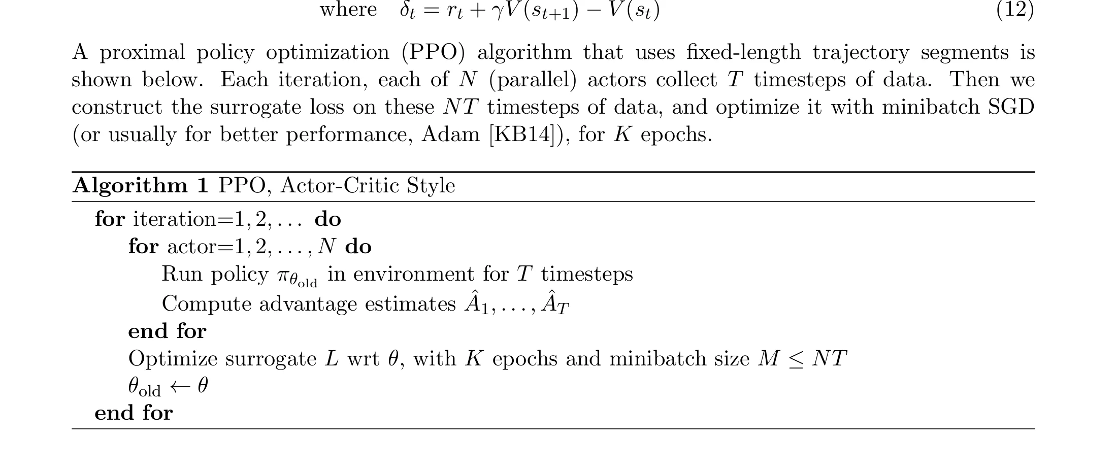
Algorithm 1 presents the standard PPO Actor-Critic workflow. The core steps are:
- 🔄 Collect data: $N$ parallel actors interact with the environment using policy $\pi_{\theta_{old}}$, each collecting $T$ timesteps of data;
- 📊 Compute advantages: Use GAE to compute advantage estimates $\hat{A}_1, \ldots, \hat{A}_T$ over the $NT$ timesteps;
- 🎯 Multi-epoch optimization: Optimize $L^{CLIP}$ over the collected data using $K$ epochs of minibatch SGD;
- 🔁 Update parameters: $\theta_{old} \leftarrow \theta$, proceed to the next iteration.
💡 Key Design Decision: PPO performs multiple epochs of optimization on a single batch of data — in stark contrast to VPG's "one batch, one update." This is the fundamental reason for PPO's dramatically improved sample efficiency. The clipping mechanism ensures that multiple rounds of updates do not cause the policy to drift too far.
6. Experimental Results 🧪
6.1 Ablation Study of Surrogate Objectives
The paper first conducts an ablation study comparing various surrogate objective variants across 7 MuJoCo continuous control tasks:
| Algorithm Variant | Average Normalized Score |
|---|---|
| No clipping or penalty | -0.39 |
| Clipping, $\epsilon = 0.2$ | 0.82 |
| Clipping, $\epsilon = 0.1$ | 0.76 |
| Clipping, $\epsilon = 0.3$ | 0.69 |
| Adaptive KL, $d_{targ}=0.01$ | 0.73 |
| Adaptive KL, $d_{targ}=0.003$ | 0.68 |
| Fixed KL, $\beta = 1$ | 0.56 |
Data from Table 1 of the paper. Higher scores are better (random policy = 0, best result = 1).
Key findings:
- 🔴 No clipping/penalty: Directly optimizing $L^{CPI}$ leads to severe performance degradation (score -0.39), confirming that multi-step optimization must be paired with a constraint mechanism;
- 🟢 PPO Clip ($\epsilon=0.2$): The best-performing variant (0.82), validating the effectiveness of the clipping mechanism;
- 🟡 Adaptive KL penalty: Outperforms fixed KL penalty but falls short of the clipping approach.
6.2 MuJoCo Continuous Control Comparison
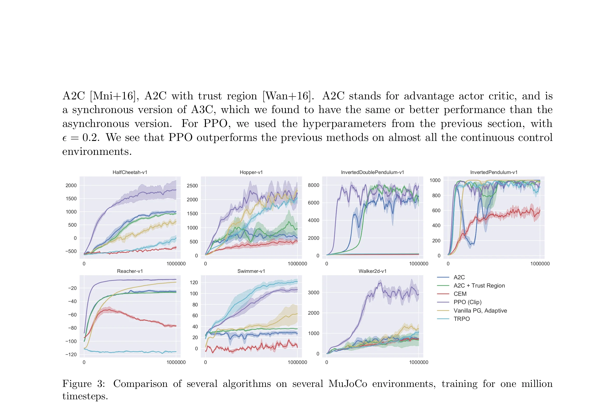
Figure 3 compares PPO against TRPO, A2C, CEM, and other algorithms across 7 MuJoCo tasks. Across all 7 environments, PPO (purple curve) is either the best or very close to the best. Notable observations:
- On Walker2d and HalfCheetah, PPO significantly outperforms TRPO;
- On InvertedPendulum, all methods converge rapidly, but PPO converges more stably;
- PPO's improvement over A2C and VPG is substantial across most environments.
6.3 3D Humanoid Robot Control
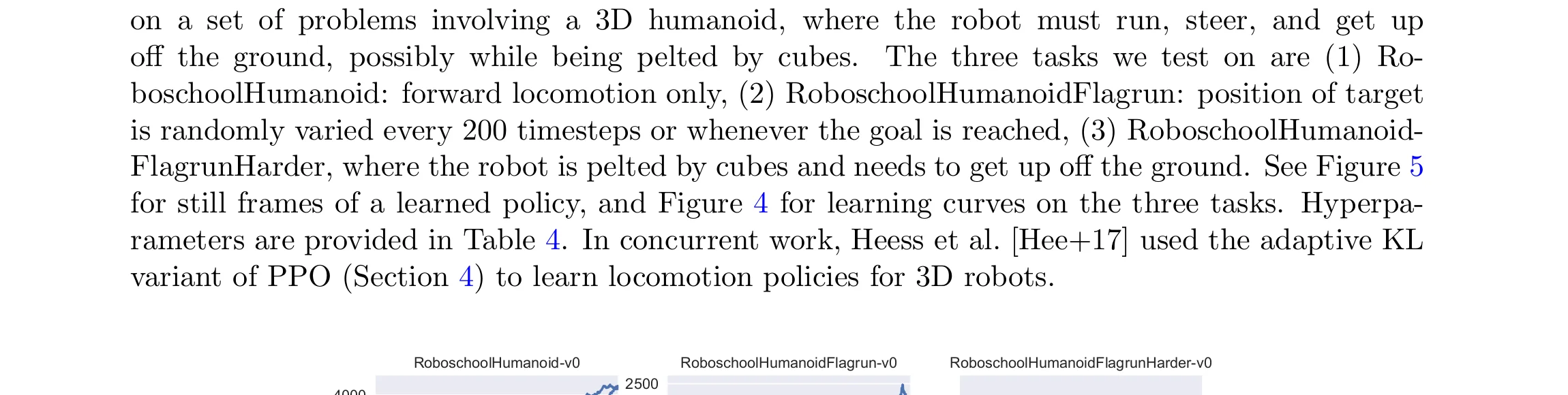
Figure 4 shows PPO's learning curves on three complex 3D humanoid control tasks (using the Roboschool environment):
- RoboschoolHumanoid: Basic forward locomotion;
- RoboschoolHumanoidFlagrun: Running toward randomly changing target positions;
- RoboschoolHumanoidFlagrunHarder: A harder variant where the robot is pelted with cubes and must get back up.
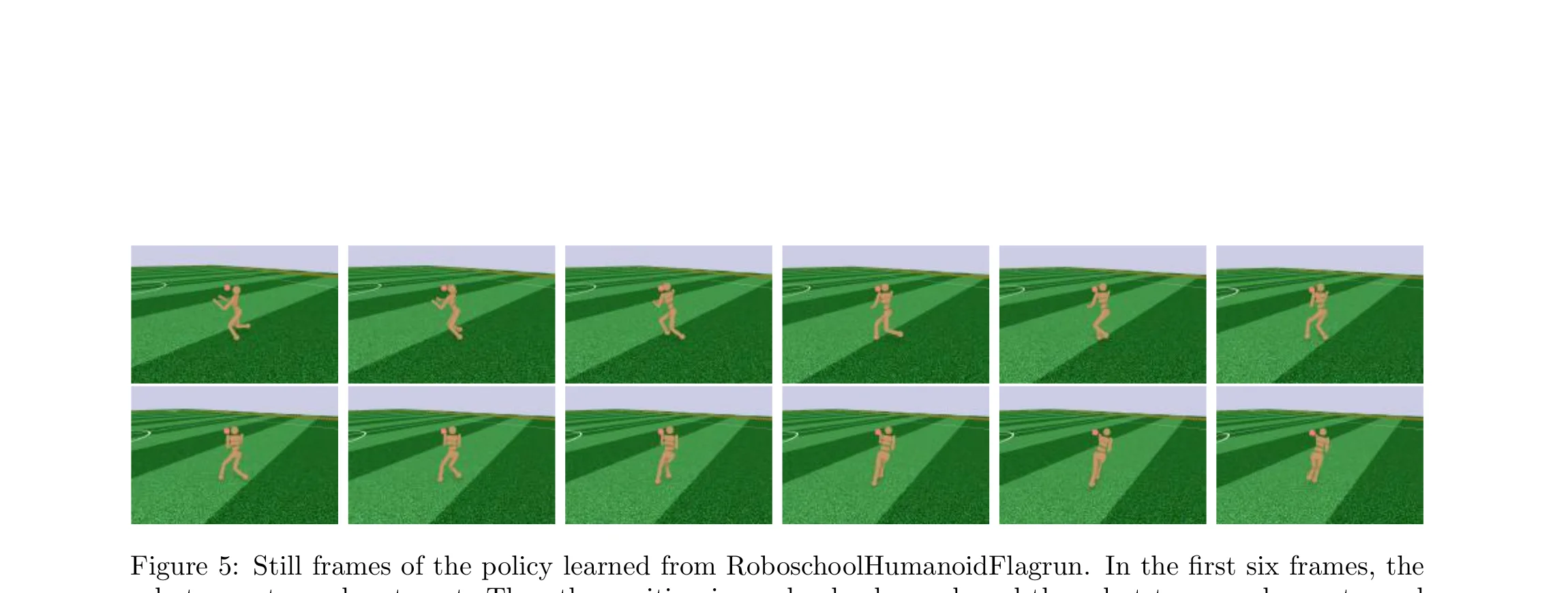
Figure 5 shows the learned policy from the RoboschoolHumanoidFlagrun task. In the first six frames, the robot runs toward a target. The target position is then randomly changed, and the robot turns and runs toward the new target. This demonstrates PPO's ability to learn robust locomotion policies in extremely high-dimensional action spaces.
6.4 Atari Game Benchmark
Comparing PPO against A2C and ACER on 49 Atari games:
| Scoring Metric | A2C | ACER | PPO |
|---|---|---|---|
| Avg. episode reward over all of training | 1 | 18 | 30 |
| Avg. episode reward over last 100 episodes | 1 | 28 | 19 |
PPO overwhelmingly outperforms A2C on "average reward over all training" (30:1), indicating faster learning. On "final performance," ACER slightly edges ahead (28:19), but considering that ACER is a substantially more complex algorithm (incorporating experience replay, bias correction, etc.), PPO's combination of simplicity and strong performance represents an extremely attractive trade-off.
7. Conclusion and Impact 🏆
PPO's contributions can be distilled into three points:
7.1 Algorithmic Innovation: The Clipped Surrogate Objective
Through the elegantly simple objective $\min(r_t(\theta) \hat{A}_t, \ \text{clip}(r_t(\theta), 1-\epsilon, 1+\epsilon) \hat{A}_t)$, PPO achieves a trust-region-like effect. The key aspects are:
- 🎯 Implicit constraint: No need for explicit KL divergence constraints or penalties — clipping naturally bounds the magnitude of policy updates;
- 📉 Pessimistic lower bound: The $\min$ operation ensures the objective never overestimates improvement in "dangerous" update directions;
- 🔧 First-order method: The entire optimization uses only stochastic gradient ascent — no conjugate gradients or line search required.
7.2 Engineering Practicality
PPO surpasses TRPO in several critical dimensions:
- 💻 Code implementation: Only a few lines of code change from vanilla policy gradient;
- 🏗️ Architectural compatibility: Supports policy-value network parameter sharing, dropout, auxiliary tasks, and other modern neural network design patterns;
- ⚡ Training efficiency: Multi-epoch updates dramatically improve sample utilization;
- 🎛️ Hyperparameter robustness: $\epsilon = 0.2$ works well across the vast majority of tasks.
7.3 Enduring Influence
Since its publication in 2017, PPO has become one of the most widely used algorithms in deep reinforcement learning:
- 🤖 OpenAI Five (Dota 2): trained using PPO;
- 🎮 OpenAI's Hide-and-Seek and Rubik's Cube robot hand — iconic projects built on PPO;
- 🚀 RLHF (Reinforcement Learning from Human Feedback): PPO is the core RL optimization algorithm in training ChatGPT and InstructGPT;
- 📚 Teaching standard: PPO is now a staple of virtually every reinforcement learning curriculum.
Looking back from 2026, PPO became a classic not because it is theoretically more elegant than TRPO — quite the opposite, TRPO's theoretical guarantees are more rigorous — but because it solved the most critical practical problem using the simplest engineering approach. The best algorithm is not necessarily the most complex one, but the one that achieves the greatest benefit with the least complexity. This is perhaps the most important lesson PPO imparts to the entire machine learning community.
8. Key Formula Reference 📋
| Formula | Expression | Purpose |
|---|---|---|
| Probability Ratio | $r_t(\theta) = \frac{\pi_\theta(a_t|s_t)}{\pi_{\theta_{old}}(a_t|s_t)}$ | Measuring policy change |
| CPI Objective | $L^{CPI}(\theta) = \hat{\mathbb{E}}_t[r_t(\theta)\hat{A}_t]$ | Unconstrained surrogate |
| PPO Clip | $L^{CLIP}(\theta) = \hat{\mathbb{E}}_t[\min(r_t\hat{A}_t, \text{clip}(r_t, 1-\epsilon, 1+\epsilon)\hat{A}_t)]$ | 🎯 Core innovation |
| KL Penalty | $L^{KLPEN}(\theta) = \hat{\mathbb{E}}_t[r_t\hat{A}_t - \beta \ \text{KL}]$ | Alternative approach |
| Combined Loss | $L^{CLIP+VF+S} = \hat{\mathbb{E}}_t[L^{CLIP} - c_1 L^{VF} + c_2 S]$ | Actor-Critic training |
| GAE | $\hat{A}_t = \sum_{l=0}^{\infty}(\gamma\lambda)^l \delta_{t+l}$ | Advantage estimation |
| TD Error | $\delta_t = r_t + \gamma V(s_{t+1}) - V(s_t)$ | Temporal-difference error |
Note: All figures in this article were extracted from the original paper PDF (arXiv:1707.06347v2). Copyright belongs to the original authors.
References:
- Schulman, J., Wolski, F., Dhariwal, P., Radford, A., & Klimov, O. (2017). Proximal Policy Optimization Algorithms. arXiv:1707.06347v2.
- Schulman, J., Levine, S., Abbeel, P., Jordan, M., & Moritz, P. (2015). Trust Region Policy Optimization. ICML 2015.
- Schulman, J., Moritz, P., Levine, S., Jordan, M., & Abbeel, P. (2015). High-Dimensional Continuous Control Using Generalized Advantage Estimation. arXiv:1506.02438.
- Kakade, S., & Langford, J. (2002). Approximately Optimal Approximate Reinforcement Learning. ICML 2002.
- Mnih, V., et al. (2016). Asynchronous Methods for Deep Reinforcement Learning. ICML 2016.